Semigroup Kernels on Measures

Semigroup Kernels on Measures

Marco Cuturi [email protected]

Ecole des Mines de Paris 35 rue Saint Honor´e

77305 Fontainebleau, France; Institute of Statistical Mathematics

4-6-7 Minami-Azabu, Minato-Ku, Tokyo, Japan

Kenji Fukumizu [email protected]

Institute of Statistical Mathematics

4-6-7 Minami-Azabu, Minato-Ku, Tokyo, Japan

Jean-Philippe Vert [email protected]

Ecole des Mines de Paris 35 rue Saint Honor´e

77305 Fontainebleau, France

Editor: John Lafferty

Abstract

We present a family of positive definite kernels on measures, characterized by the fact that the value of the kernel between two measures is a function of their sum. These kernels can be used to derive kernels on structured objects, such as images and texts, by representing these objects as sets of components, such as pixels or words, or more generally as measures on the space of components. Several kernels studied in this work make use of common quantities defined on measures such as entropy or generalized variance to detect similarities. Given an a priori kernel on the space of components itself, the approach is further extended by restating the previous results in a more efficient and flexible framework using the “kernel trick”. Finally, a constructive approach to such positive definite kernels through an integral representation theorem is proved, before presenting experimental results on a benchmark experiment of handwritten digits classification to illustrate the validity of the approach.

Keywords: kernels on measures, semigroup theory, Jensen divergence, generalized variance, reproducing kernel Hilbert space

1. Introduction

structured objects. This situation motivates the proposal of various kernels, either tuned and trained to be efficient on specific applications or useful in more general cases.

One possible approach to kernel design for such complex objects consists in representing them by sets of basic components easier to manipulate, and designing kernels on such sets. Such basic components can typically be subparts of the original complex objects, obtained by exhaustive enu-meration or random sampling. For example, a very common way to represent a text for applications such as text classification and information retrieval is to break it into words and consider it as a bag of words, that is, a finite set of weighted terms. Another possibility is to extract all fixed-length blocks of consecutive letters and represent the text by the vector of counts of all blocks (Leslie et al., 2002), or even to add to this representation additional blocks obtained by slight modifications of the blocks present in the text with different weighting schemes (Leslie et al., 2003). Similarly, a grey-level digitalized image can be considered as a finite set of points ofR3 _{where each point (x,y,I)} stands for the intensity I displayed on the pixel(x,y)in that image (Kondor and Jebara, 2003).

Once such a representation is obtained, different strategies have been adopted to design kernels on these descriptions of complex objects. When the set of basic components is finite, this repre-sentation amounts to encode a complex object as a finite-dimensional vector of counters, and any kernel for vectors can be then translated to a kernel for complex object through this feature represen-tation (Joachims, 2002, Leslie et al., 2002, 2003). For more general situations, several authors have proposed to handle such weighted lists of points by first fitting a probability distribution to each list, and defining a kernel between the resulting distributions (Lafferty and Lebanon, 2002, Jebara et al., 2004, Kondor and Jebara, 2003, Hein and Bousquet, 2005). Alternatively, Cuturi and Vert (2005) use a parametric family of densities and a Bayesian framework to define a kernel for strings based on the mutual information between their sets of variable-length blocks, using the concept of mutual information kernels (Seeger, 2002). Finally, Wolf and Shashua (2003) recently proposed a formulation rooted in kernel canonical correlation analysis (Bach and Jordan, 2002, Melzer et al., 2001, Akaho, 2001) which makes use of the principal angles between the subspaces generated by the two sets of points to be compared when considered in a feature space.

We explore in this contribution a different direction to kernel design for weighted lists of basic components. Observing that such a list can be conveniently represented by a molecular measure on the set of basic components, that is a weighted sum of Dirac measures, or that the distribution of points might be fitted by a statistical model and result in a density on the same set, we formally focus our attention on the problem of defining a kernel between finite measures on the space of basic components. More precisely, we explore the set of kernels between measures that can be expressed as a function of their sum, that is:

k(µ,µ0) =ϕ(µ+µ0). (1)

The rationale behind this formulation is that if two measures or sets of points µ and µ0overlap, then it is expected that the sum µ+µ0 is more concentrated and less scattered than if they do not. As a result, we typically expectϕto quantify the dispersion of its argument, increasing when it is more concentrated. This setting is therefore a broad generalization of the observation by Cuturi and Vert (2005) that a valid kernel for strings, seen as bags of variable-length blocks, is obtained from the compression rate of the concatenation of the two strings by a particular compression algorithm.

densities. As expected, we prove that several functionsϕthat quantify the dispersion of measures through their entropy or through their variance matrix result in valid p.d. kernels. Using entropy to compare two measures is not a new idea (Rao, 1987) but it was recently restated within different frameworks (Hein and Bousquet, 2005, Endres and Schindelin, 2003, Fuglede and Topsøe, 2004). We introduce entropy in this paper slightly differently, noting that it is a semigroup negative definite function defined on measures. On the other hand, the use of generalized variance to derive a positive definite kernel between measures as proposed here is new to our knowledge. We further show how such kernels can be applied to molecular measures through regularization operations. In the case of the kernel based on the spectrum of the variance matrix, we show how it can be applied implicitly for molecular measures mapped to a reproducing kernel Hilbert space when a p.d. kernel on the space of basic components is provided, thanks to an application of the “kernel trick”.

Besides these examples of practical relevance, we also consider the question of characterizing

all functionsϕthat lead to a p.d. kernel through (1). Using the general theory of semigroup kernels

we state an integral representation of such kernels and study the semicharacters involved in this representation. This new result provides a constructive characterization of such kernels, which we briefly explore by showing that Bayesian mixtures over exponential models can be seen as natural functionsϕthat lead to p.d. kernels, thus making the link with the particular case treated by Cuturi and Vert (2005).

This paper is organized as follows. We first introduce elements of measure representations of weighted lists and define the semigroup formalism and the notion of semigroup p.d. kernel in Sec-tion 2. SecSec-tion 3 contains two examples of semigroup p.d. kernels, which are however usually not defined for molecular measures: the entropy kernel and the inverse generalized variance (IGV) kernel. Through regularization procedures, practical applications of such kernels on molecular mea-sures are proposed in Section 4, and the approach is further extended by kernelizing the IGV through an a priori kernel defined itself on the space of components in Section 5. Section 6 contains the gen-eral integral representation of semigroup kernels and Section 7 makes the link between p.d. kernels and Bayesian posterior mixture probabilities. Finally, Section 8 contains an empirical evaluation of the proposed kernels on a benchmark experiment of handwritten digits classification.

2. Notations and Framework: Semigroup Kernels on Measures

In this section we set up the framework and notations of this paper, in particular the idea of semi-group kernel on the semisemi-group of measures.

2.1 Measures on Basic Components

We model the space of basic components by a Hausdorff space(

X

,

B

,ν) endowed with its Borel

σ-algebra and a Borel dominant measureν. A positive Radon measure µ is a positive Borel measure which satisfies (i)µ(C)<+∞for any compact subset C_⊆

X

and(ii)µ(B) =sup_{µ(C)_|C_⊆B,C

compact}for any B∈

B

(see for example Berg et al. (1984) for the construction of Radon measures on Hausdorff spaces). The set of positive bounded (i.e., µ(

X

)<+∞) Radon measures on

X

is de-noted by Mb₊(

X

). We introduce the subset of Mb₊(

X

)of molecular (or atomic) measures Mol+(

X

), namely measures such that

is finite, and we denote by δx ∈Mol+(

X

) the molecular (Dirac) measure of weight 1 on x. For a molecular measure µ, an admissible base of µ is a finite listγof weighted points of

X

, namely

γ= (xi,ai)di=1, where xi∈

X

and ai>0 for 1≤i≤d, such that µ=∑di=1aiδxi. We write in that case |γ|=∑d

i=1ai and l(γ) =d. Reciprocally, a measure µ is said to be the image measure of a list of weighted elementsγif the previous equality holds. Finally, for a Borel measurable function f _∈RX and a Borel measure µ, we write µ[f] =R

X f dµ.

2.2 Semigroups and Sets of Points

We follow in this paper the definitions found in Berg et al. (1984), which we now recall. An Abelian

semigroup(

S

,+)is a nonempty set S endowed with an associative and commutative composition

+and a neutral element 0. Referring further to the notations used in Berg et al. (1984), note that we will only use auto-involutive semigroups in this paper, and will hence not discuss other semigroups which admit different involutions.

A functionϕ:

S

_→R_{is called a positive definite (resp. negative definite, n.d.) function on the} semigroup(S,+)if(s,t)_7→ϕ(s+t)is a p.d. (resp. n.d.) kernel on

S

_×

S

. The symmetry of the kernel being ensured by the commutativity of+, the positive definiteness is equivalent to the fact that the inequality

N

∑

i,j=1

cicjϕ(xi+xj)≥0

holds for any N_∈N_{,(x1, . . . ,xN)∈}

S

N _and(c

1. . . ,cn)∈RN. Using the same notations, and adding the additional condition that∑n_i=1ci=0 yields the definition of negative definiteness asϕsatisfying

now

N

∑

i,j=1

cicjϕ(xi+xj)≤0.

Hence semigroup kernels are real-valued functionsϕdefined on the set of interest

S

, the similarity between two elements s,t of

S

being just the value taken by that function on their composition, namelyϕ(s+t).

Recalling our initial goal to quantify the similarity between two complex objects through finite weighted lists of elements in

X

, we note that(

P

(

X

),_∪)the set of subsets of

X

equipped with the usual union operator_∪is a semigroup. Such a semigroup might be used as a feature representation for complex objects by mapping an object to the set of its components, forgetting about the weights. The resulting representation would therefore be an element of

P

(

X

). A semigroup kernel k on

P

(

X

) measuring the similarity of two sets of points A,B_∈

P

(

X

) would use the value taken by a given p.d. function ϕ on their union, namely k(A,B) =ϕ(A_∪B). However we put aside this framework for two reasons. First, the union composition is idempotent (i.e., for all A in

P

(

X

), we have A_∪A=A) which as noted in Berg et al. (1984, Proposition 4.4.18) drastically restricts the class

of possible p.d. functions. Second, such a framework defined by sets would ignore the frequency (or weights) of the components described in lists, which can be misleading when dealing with finite sets of components. Other problematic features would include the fact that k(A,B)would be constant when B⊂A regardless of its characteristics, and that comparing sets of very different sizes should

be difficult.

focus now on the Abelian semigroup(M₊b(

X

),+)to define kernels between lists of weighted points. This representation is richer than the one suggested in the previous paragraph in the semigroup (

P

(

X

),_∪) to consider the merger of two lists. First it performs the union of the supports; second the sum of such molecular measures also adds the weights of the points common to both measures, with a possible renormalization on those weights. Two important features of the original list are however lost in this mapping: the order of its elements and the original frequency of each element within the list as a weighted singleton. We assume for the rest of this paper that this information is secondary compared to the one contained in the image measure, namely its unordered support and the overall frequency of each point in that support. As a result, we study in the following sections p.d. functions on the semigroup(Mb

+(

X

),+), in particular on molecular measures, in order to define kernels on weighted lists of simple components.

X

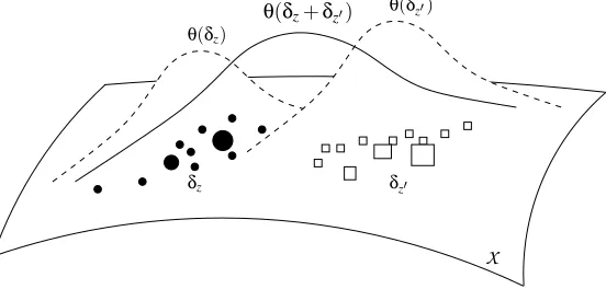
θ(δz)

θ(δz0)

θ(δz+δz0)

δz δz0

Figure 1: Measure representations of two lists z and z0. Each element of z (resp. z0) list is repre-sented by a black circle (resp. a white square), the size of which represents the associated weight. Five measures of interest are represented: the image measuresδzandδz0 of those

weighted finite lists, the smoothed density estimatesθ(δz)andθ(δz0)of the two lists of

points, and the smoothed density estimateθ(δz+δz0)of the union of both lists.

Before starting the analysis of such p.d. functions, it should however be pointed out that several interesting semigroup p.d. kernels on measures are not directly applicable to molecular measures. For example, the first function we study below is only defined on the set of absolutely continuous measures with finite entropy. In order to overcome this limitation and be able to process complex objects in such situations, it is possible to think about alternative strategies to represent such objects by measures, as illustrated in Figure 1:

• The molecular measuresδzandδz0 as the image measures corresponding to the two weighted

sets of points of z and z0, where dots and squares represent the different weights applied on each points;

• Alternatively, smoothed estimates of these distributions obtained for example by non-parametric or parametric statistical density estimation procedures, and represented byθ(δz) andθ(δz0)

of densities (through maximum likelihood for instance) this can also be seen as a prior belief assumed on the distribution of the objects;

• Finally, a smoothed estimate of the sumδz+δz0 corresponding to the merging of both lists,

represented byθ(δz+δz0), can be considered. Note thatθ(δz+δz0)might differ fromθ(δz) +

θ(δz0).

A kernel between two lists of points can therefore be derived from a p.d. function on(M₊b(

X

),+) in at least three ways:

k(z,z0) =



 

 

ϕ(δz+δz0), usingϕdirectly on molecular measures,

ϕ(θ(δz) +θ(δz0)), usingϕon smoothed versions of the molecular measures,

ϕ(θ(δz+δz0)), evaluatingϕon a smoothed version of the sum.

The positive definiteness of ϕ on M₊b(

X

) ensures positive definiteness of k only in the first two cases. The third expression can be seen as a special case of the first one, where we highlight the usage of a preliminary mapping on the sum of two measures; in that case ϕ_◦θshould in fact be p.d. on(M₊b(

X

),+), or at least(Mol+(

X

),+). Having defined the set of representations on which we will focus in this paper, namely measures on a set of components, we propose in the following section two particular cases of positive definite functions that can be computed through an addition between the considered measures. We then show how those quantities can be computed in the case of molecular measures in Section 4.

3. The Entropy and Inverse Generalized Variance Kernels

In this section we present two basic p.d. semigroup kernels for measures, motivated by a common intuition: the kernel between two measures should increase when the sum of the measures gets more “concentrated”. The two kernels differ in the way they quantify the concentration of a mea-sure, using either its entropy or its variance. They are therefore limited to a subset of measures, namely the subset of measures with finite entropy and the subset of sub-probability measures with non-degenerated variance, but are extended to a broader class of measures, including molecular measures, in Section 4.

3.1 Entropy Kernel

We consider the subset of Mb₊(

X

)of absolutely continuous measures with respect to the dominant measureν, and identify in this section a measure with its corresponding density with respect toν. We further limit the subset to the set of non-negative valuedν-measurable functions on

X

with finite sum, such that

M₊h(

X

)def=_{f :

X

_→R+_{|f is}ν_{-measurable,|h(f)|<}∞_,|f|<∞_} where we write for any measurable non-negative valued function g,

h(g)def=₋

Z

(with 0 ln 0=0 by convention) and_|g_|def=R

Xg dν, consistently with the notation used for measures.

If g is such that_|g_|=1, h(g)is its differential entropy. Using the following inequalities,

(a+b)ln(a+b)_≤a ln a+b ln b+ (a+b)ln 2, by convexity of x_7→x ln x, (a+b)ln(a+b)_≥a ln a+b ln b,

we have that(Mh₊(

X

),+)is an Abelian semigroup since for f,f0in Mh₊(

X

)we have that h(f+f0) is bounded by integrating pointwise the inequalities above, the boundedness of_|f+f0_|being also ensured. Following Rao (1987) we consider the quantity

J(f,f0)def=h(f+f0 2 )−

h(f) +h(f0)

2 , (2)

known as the Jensen divergence (or Jensen-Shannon divergence) between f and f0, which as noted by Fuglede and Topsøe (2004) can be seen as a symmetrized version of the Kullback-Leibler (KL) divergence D, since

J(f,f0) =1 2D(f||

f+f0

2 ) + 1 2D(f

0_||f+f0 2 ).

The expression of Equation (2) fits our framework of devising semigroup kernels, unlike the direct use of the KL divergence (Moreno et al., 2004) which is neither symmetric nor negative definite. As recently shown in Endres and Schindelin (2003) and ¨Osterreicher and Vajda (2003),√J is a metric

on M₊h(

X

)which is a direct consequence of J’s negative definiteness proven below, through Berg et al. (1984, Proposition 3.3.2) for instance. The Jensen-Divergence was also recently reinterpreted as a special case of a wider family of metrics on M₊b(

X

)derived from a particular family of Hilber-tian metrics onR_{+ as presented in Hein and Bousquet (2005). The comparison between two} den-sities f,f0 is in that case performed by integrating pointwise the squared distance d2(f(x),f0(x)) between the two densities over

X

, using for d a distance chosen among a suitable family of metrics in R_{+ to ensure that the final value is independent of the dominant measure} ν_{. The considered} family for d is described in Fuglede and Topsøe (2004) through two parameters, a family of which the Jensen Divergence is just a special case as detailed in Hein and Bousquet (2005). The latter work shares with this paper another similarity, which lies in the “kernelization” of such quanti-ties defined on measures through a prior kernel on the space of components, as will be reviewed in Section 5. However, of all the Hilbertian metrics introduced in Hein and Bousquet (2005), the Jensen-Divergence is the only one that can be related to the semigroup framework used throughout this paper.

Note finally that a positive definite kernel k is said to be infinitely divisible if₋ln k is a negative definite kernel. As a consequence, any positive exponentiation kβ,β>0 of an infinitely divisible kernel is a positive definite kernel.

Proposition 1 h is a negative definite function on the semigroup Mh₊(

X

). As a consequence e−h

is a positive definite function on M₊h(

X

) and its normalized counterpart, khdef=e−J is an infinitely divisible positive definite kernel on Mh₊(

X

)_×M₊h(

X

).

Proof It is known that the real-valued function r : y_{7→ −}y ln y is n.d. onR_{+as a semigroup endowed} with addition (Berg et al., 1984, Example 6.5.16). As a consequence the function f _7→r_◦f is n.d.

remains negative definite. This allows first to prove that h(f+₂f0)is also n.d. through the identity

h(f+₂f0) = 1₂h(f+f0) +ln 2₂ (_|f_|+_|f0_|). Subtracting the normalization factor 1₂(h(f) +h(f0))gives the negative definiteness of J. This finally yields the positive definiteness of khas the exponential of

the negative of a n.d. function through Schoenberg’s theorem (Berg et al., 1984, Theorem 3.2.2).

Note that only e−h is a semigroup kernel strictly speaking, since e−J involves a normalized sum (through the division by 2) which is not associative. While both e−hand e−J can be used in practice on non-normalized measures, we name more explicitly kh=e−J the entropy kernel, because what

it indeed quantifies when f and f0 are normalized (i.e., such that_|f_|=_|f0_|=1) is the difference of the average of the entropy of f and f0from the entropy of their average. The subset of absolutely continuous probability measures on(

X

,ν)with finite entropies, namelyf_∈M₊h(

X

),s.t._|f_|=1 is not a semigroup since it is not closed by addition, but we can nonetheless define the restriction of J and hence khon it to obtain a p.d. kernel on probability measures inspired by semigroup formalism.

3.2 Inverse Generalized Variance Kernel

We assume in this subsection that

X

is an Euclidian space of dimension n endowed with Lebesgue’s measure ν. Following the results obtained in the previous section, we propose under these re-strictions a second semigroup p.d. kernel between measures which uses generalized variance. The generalized variance of a measure, namely the determinant of its variance matrix, is a quantity ho-mogeneous to a volume in

X

. This volume can be interpreted as a typical volume occupied by a measure when considering only its second order moments, making it hence a useful quantification of its dispersion. Besides being easy to compute in the case of molecular measures, this quantity is also linked to entropy if we consider that for normal laws

N

(m,Σ)the following relation holds:

1

√

detΣ∝e

−h(N(m,Σ))_.

Through this observation, we note that considering the Inverse of the Generalized Variance (IGV) of a measure is equivalent to considering the value taken by e−2hon its maximum likelihood normal law. We will put aside this interpretation in this section, before reviewing it with more care in Section 7.

Let us define the variance operator on measures µ with finite first and second moment of M₊b(

X

) as

Σ(µ)def=µ[xx>]₋µ[x]µ[x]>.

Note thatΣ(µ)is always a positive semi-definite matrix when µ is a sub-probability measure, that is when_|µ_{| ≤}1, since

Σ(µ) =µ[(x₋µ[x]) (x₋µ[x])>] + (1_{− |}µ_|)µ[x]µ[x]>.

We call detΣ(µ)the generalized variance of a measure µ, and say a measure µ is non-degenerated if detΣ(µ)is non-zero, meaning thatΣ(µ)is of full rank. The subset of M₊b(

X

)of such measures with total weight equal to 1 is denoted by M₊v(

X

); M₊v(

X

)is convex through the following proposition:

Proposition 2 Mv₊(

X

)def=

Proof We use the following identity,

Σ (1₋λ)µ+λµ0

= (1₋λ)Σ(µ) +λΣ(µ0) +λ(1₋λ) µ[x]₋µ0[x]

µ[x]₋µ0[x]>

,

to derive thatΣ((1₋λ)µ+λµ0) is a (strictly) positive-definite matrix as the sum of two positive semi-definite matrices and a strictly positive definite matrixΣ(µ).

M₊v(

X

)is not a semigroup, since it is not closed under addition. However we will work in this case on the mean of two measures in the same way we used their standard addition in the semigroup framework of Mb₊(

X

).

Proposition 3 The real-valued kernel kvdefined on elements µ,µ0of M+v(

X

)as

kv(µ,µ0) =

1

detΣ(µ+₂µ0)

is positive definite.

Proof Let y be an element of

X

. For any N ∈N_{, any c1}, ...,cN ∈R_{such that} ∑i_ci =0 and any

µ1, ...,µN∈Mv+(

X

)we have

∑

i,j

cicjy>Σ( µi+µj

2 )y=

∑

_i,jcicjy > 1

2µi[xx >_{] +}1

2µj[xx >_]−

1 4

µi[x]µi[x]>+µj[x]µj[x]>+µj[x]µi[x]>+µi[x]µj[x]>

!

y

=₋1

4

∑

_i,jcicjy >_µ

j[x]µi[x]>+µi[x]µj[x]>

y

=₋1

2

∑

_i ciy >_µi[x]

!2 ≤0,

making thus the function µ,µ0_7→y>Σ(µ+₂µ0)y negative-definite for any y_∈

X

. Using again Schoen-berg’s theorem (Berg et al., 1984, Theorem 3.2.2) we have that µ,µ0_7→e−y>Σ(µ+µ

0

2 )yis positive

defi-nite and so is the sum 1 (2π)n2

R

Xe−y

>_Σ(µ+µ0

2 )yν(dy)which is equal to 1/ q

detΣ(µ+₂µ)ensuring thus the positive-definiteness of kvas its square.

Both entropy and IGV kernels are defined on subsets of M₊b(

X

). Since we are most likely to use them on molecular measures or smooth measures (as discussed in Section 2.2), we present in the following section practical ways to apply them in that framework.

4. Semigroup Kernels on Molecular Measures

finite spaces), and they have therefore no entropy; we solve this problem by mapping them into

Mh₊(

X

) through a smoothing kernel. In the case of the IGV, the estimates of variances might be poor if the number of points in the lists is not large enough compared to the dimension of the Euclidean space; we perform in that case a regularization by adding a unit-variance correlation matrix to the original variance. This regularization is particularly important to pave the way to the kernelized version of the IGV kernel presented in the next section, when

X

is not Euclidian but simply endowed with a prior kernelκ.

The application of both the entropy kernel and the IGV kernel to molecular measures requires a previous renormalization to set the total mass of the measures to 1. This technical renormalization is also beneficial, since it allows a consistent comparison of two weighted lists even when their size and total mass is very different. All molecular measures in this section, and equivalently all admissible bases, will hence be supposed to be normalized such that their total weight is 1, and Mol1₊(

X

)denotes the subset of Mol+(

X

)of such measures.

4.1 Entropy Kernel on Smoothed Estimates

We first define the Parzen smoothing procedure which allows to map molecular measures onto measures with finite entropy:

Definition 4 Let κ be a probability kernel on

X

with finite entropy, i.e., a real-valued function defined on

X

2_{such that for any x∈}

_X

_{,κ(x,·): y7→κ(x,y)satisfiesκ(x,·)∈M}h

+(

X

)and|κ(x,·)|=1.

Theκ-Parzen smoothed measure of µ is the probability measure whose density with respect toνis θκ(µ), where

θκ: Mol1₊(

X

)_−→M₊h(

X

)

µ_7→

∑

x∈supp µ

µ(x)κ(x,_·).

Note that for any admissible base (xi,ai)dk=1 of µ we have thatθκ(µ) =∑di=1aiκ(xi,·). Once this

mapping is defined, we use the entropy kernel to propose the following kernel on two molecular measures µ and µ0,

kκ_h(µ,µ0) =e−J(θκ(µ),θκ(µ0)).

As an example, let

X

be an Euclidian space of dimension n endowed with Lebesgue’s measure, andκthe isotropic Gaussian RBF kernel on that space, namely

κ(x,y) = 1 (2πσ)n2

e−k

x−yk2

2σ2 .

Given two weighted lists z and z0 of components in

X

, θκ(δz) and θκ(δz0) are thus mixtures of

Gaussian distributions on

X

. The resulting kernel computes the entropy ofθ_κ(δz)andθ_κ(δz0)taken

separately and compares it with that of their mean, providing a positive definite quantification of their overlap.

4.2 Regularized Inverse Generalized Variance of Molecular Measures

In the case of a molecular measure µ defined on an Euclidian space

X

of dimension n, the variance

of

X

:

Σ(µ) =µ[xx>]₋µ[x]µ[x]> =

d

∑

i=1

aixix>_i −

d

∑

i=1

aixi

!

d

∑

i=1

aixi

!>

,

where we use an admissible baseγ= (xi,ai)di=1 of µ to give a matrix expression ofΣ(µ), with all points xi expressed as column vectors. Note that this matrix expression, as would be expected from

a function defined on measures, does not depend on the chosen admissible base. Given such an admissible base, let X_γ= [xi]i=1..d be the n×d matrix made of all column vectors xi and ∆γ the

diagonal matrix of weights of γtaken in the same order(ai)1_≤ı≤d. If we write Id for the identity

matrix of rank d and d,dfor the d×d matrix composed of ones, we have for any baseγof µ that:

Σ(µ) =Xγ(∆γ−∆γ d,d∆γ)X_γ>,

which can be rewritten as

Σ(µ) =Xγ(Id₋∆γ d,d)∆γ(Id− d,d∆γ)Xγ>,

noting that(∆_γ d,d)2=∆γ d,d since trace∆γ=1.

The determinant ofΣ(µ)can be equal to zero when the size of the support of µ is smaller than

n, the dimension of

X

, or more generally when the linear span of the points in the support of µ

does not cover the whole space

X

. This problematic case is encountered in Section 5 when we consider kernelized versions of the IGV, using an embedding of

X

into a functional Hilbert space of potentially infinite dimension. Mapping an element of Mol1₊(

X

)into M₊v(

X

)by adding to it any element of Mv₊(

X

)through Proposition 2 would work as a regularization technique; for an arbitrary

ρ_∈Mv₊(

X

)and a weightλ_∈[0,1)we could use the kernel defined as

µ,µ0_7→ 1

detΣ

λµ+µ0

2 + (1−λ)ρ

.

We use in this section a different strategy inspired by previous works (Fukumizu et al., 2004, Bach and Jordan, 2002) further motivated in the case of covariance operators on infinite dimensional spaces as shown by Cuturi and Vert (2005). The considered regularization consists in modifying directly the matrixΣ(µ)by adding a small diagonal componentηInwhereη>0 so that its spectrum never vanishes. When considering the determinant of such a regularized matrixΣ(µ) +ηInthis is equivalent to considering the determinant of _η1Σ(µ) +In up to a factor ηn, which will be a more

suitable expression in practice. We thus introduce the regularized kernel kvη defined on measures

(µ,µ0)_∈M₊b(

X

)with finite second moment as

k_vη(µ,µ0)def= 1 det

1

ηΣ

µ+µ0 2

+In

.

It is straightforward to prove that the regularized function kvη is a positive definite kernel on the

measures of M₊b(

X

)with finite second-order moments using the same proof used in Proposition 3. If we now introduce

Kγdef=hx>_i xj

i

for the d×d matrix of dot-products associated with the elements of a baseγ, and

˜

K_γdef=

"

(xi− d

∑

k=1

akxk)>(xj− d

∑

k=1

akxk)

#

1≤i,j≤d

= (Id− d,d∆γ)Kγ(Id−∆γ d,d),

for its centered expression with respect to the mean of µ, we have the following result:

Proposition 5 Let

X

be an Euclidian space of dimension n. For any µ_∈Mol1₊(

X

)and any

admis-sible baseγof µ we have

det

1

ηK˜γ∆γ+Il(γ)

=det

1

ηΣ(µ) +In

.

Proof We omit the references to µ and γ in this proof to simplify matrix notations, and write

d=l(γ). Let ˜X be the n_×d matrix[xi₋∑d_j=1ajxj]i=1..d of centered column vectors enumerated in γ, namely ˜X=X(Id−∆ d,d). We have

Σ=X˜∆X˜>,

˜

K∆=_X˜>_{X∆˜ .}

Through the singular value decomposition of ˜X∆12, it is straightforward to see that the non-zero

elements of the spectrums of matrices ˜K∆,∆12X˜>X˜∆12 andΣare identical. Thus, regardless of the

difference between n and d, we have

det

1

ηK∆˜ +Id

=det 1 η∆ 1

2_X˜>_X˜∆

1

2+_Id

=det

1

ηX∆˜ X˜>+In

=det

1

ηΣ+In

,

where the addition of identity matrices only introduces an offset of 1 for all eigenvalues.

Given two measures µ,µ0_∈Mol1₊(

X

), the following theorem can be seen as a regularized equivalent of Proposition 3 through an application of Proposition 5 to µ00= µ+₂µ0.

Theorem 6 Let

X

be an Euclidian space. The kernel kvηdefined on two measures µ,µ0of Mol1+(

X

)

as

kη_v(µ,µ0) = 1

det_η1K˜_γ∆_γ+Il(γ)

,

whereγis any admissible base of µ+₂µ0, is p.d. and independent of the choice ofγ.

Given two objects z,z0 and their respective molecular measuresδz andδz0, the computation of the

IGV for two such objects requires in practice an admissible base ofδz+δz0

2 as seen in Theorem 6. This admissible base can be chosen to be of the cardinality of the support of the mixture ofδzandδz0, or

alternatively be the simple merger of two admissible bases of z and z0with their weights divided by 2, without searching for overlapped points between both lists. This choice has no impact on the final value taken by the regularized IGV-kernel and can be arbitrated by computational considerations.

since

X

may not have a vectorial structure, and the distribution of the components may not even be well represented by Gaussians in the Euclidian case. We propose to bypass this issue and intro-duce the usage of the IGV in a more flexible framework by using the kernel trick on the previous quantities, since the IGV of a measure can be expressed only through the dot-products between the elements of the support of the considered measure.

5. Inverse Generalized Variance on the RKHS Associated with a Kernelκ

As with many quantities defined by dot-products, one is tempted to replace the usual dot-product matrix ˜K of Theorem 6 by an alternative Gram-matrix obtained through a p.d. kernel κ defined on

X

. The advantage of such a substitution, which follows the well known “kernel trick” princi-ple (Sch¨olkopf and Smola, 2002), is multiprinci-ple as it first enables us to use the IGV kernel on any non-vectorial space endowed with a kernel, thus in practice on any component space endowed with a kernel; second, it is also useful when

X

is a dot-product space where a non-linear kernel can however be used (e.g., using Gaussian kernel) to incorporate into the IGV’s computation higher-order moment comparisons. We prove in this section that the inverse of the regularized generalized variance, computed in Proposition 5 through the centered dot-product matrix ˜K_γof elements of any admissible baseγof µ, is still a positive definite quantity if we replace ˜Kγby a centered Gram-matrix

˜

K

_γ, computed through an a priori kernelκon

X

, namely

K

_γ= [κ(xi,xj)]1≤i,j≤d

˜

K

_γ= (Id− d,d∆γ)

K

γ(Id−∆γ d,d).

This substitution follows also a general principle when considering kernels on measures. The “ker-nelization” of a given kernel defined on measures to take into account a prior similarity on the components, when computationally feasible, is likely to improve its overall performance in classifi-cation tasks, as observed in Kondor and Jebara (2003) but also in Hein and Bousquet (2005) under the “Structural Kernel” appellation. The following theorem proves that this substitution is valid in the case of the IGV.

Theorem 7 Let

X

be a set endowed with a p.d. kernelκ. The kernel

k_κη(µ,µ0) = 1

det

1

η

K

˜γ∆γ+Il(γ)

, (3)

defined on two elements µ,µ0in Mol1₊(

X

)is positive definite, whereγis any admissible base ofµ+₂µ0.

Proof Let N_∈N_{, µ1, ..,µN∈Mol}1

+(

X

)and(ci)Ni=1∈RN. Let us now study the quantity∑Ni=1cicjkκη(µi,µj).

To do so we introduce by the Moore-Aronszajn theorem (Berlinet and Thomas-Agnan, 2003, p.19) the reproducing kernel Hilbert spaceΞwith reproducing kernelκindexed on

X

. The usual mapping from

X

toΞis denoted byφ, that isφ:

X

₃x_7→κ(x,_·). We define

Y

def=supp

N

∑

i=1

µi

!

⊂

X

,

the finite set which numbers all elements in the support of the N considered measures, and

ϒdef

the linear span of the elements in the image of

Y

through φ. ϒ is a vector space whose finite dimension is upper-bounded by the cardinality of

Y

. Endowed with the dot-product inherited from

Ξ, we further have thatϒis Euclidian. Given a molecular measure µ_∈Mol1₊(

Y

), letφ(µ)denote the image measure of µ inϒ, namelyφ(µ) =∑x_∈Yµ(x)δφ(x). One can easily check that any admissible base γ= (xi,ai)di=1 of µ can be used to provide an admissible base φ(γ)

def

= (φ(xi),ai)di=1 of φ(µ). The weight matrices∆γand∆_φ(γ)are identical and we further have ˜

K

γ=K˜φ(γ)by the reproducing property, where ˜K is defined by the dot-product of the Euclidian space ϒ induced by κ. As a result, we have that kη_κ(µi,µj) =kvη(φ(µi),φ(µj)) where kηv is defined on Mol1₊(ϒ), ensuring the

non-negativity

N

∑

i=1

cicjkηκ(µi,µj) = N

∑

i=1

cicjkηv(φ(µi),φ(µj))≥0

and hence positive-definiteness of kη_κ.

As bserved in the experimental section, the kernelized version of the IGV is more likely to be suc-cessful to solve practical tasks since it incorporates meaningful information on the components. Be-fore observing these practical improvements, we provide a general study of the family of semigroup kernels on M₊b(

X

)by casting the theory of integral representations of positive definite functions on a semigroup (Berg et al., 1984) in the framework of measures, providing new results and possible interpretations of this class of kernels.

6. Integral Representation of Positive Definite Functions on a Set of Measures

In this section we study a general characterization of all p.d. functions on the whole semigroup (Mb

+(

X

),+), including thus measures which are not normalized. This characterization is based on a general integral representation theorem valid for any semigroup kernel, and is similar in spirit to the representation of p.d. functions obtained on Abelian groups through Bochner’s theorem (Rudin, 1962). Before stating the main results in this section we need to recall basic definitions of semichar-acters and exponentially bounded function (Berg et al., 1984, chap. 4).

Definition 8 A real-valued functionρon an Abelian semigroup(S,+)is called a semicharacter if it satisfies the following properties:

(i) ρ(0) =1

(ii) _∀s,t_∈S,ρ(s+t) =ρ(s)ρ(t).

It follows from the previous definition and the fact that M₊b(

X

)is 2-divisible (i.e.,∀µ∈M₊b(

X

),_∃µ0∈

Mb₊(

X

) s.t. µ=2µ0) that semicharacters are nonnegative valued since it suffices to write that

ρ(µ) =ρ(µ₂)2_{. Note also that semicharacters are trivially positive definite functions on S. We} de-note by S∗ the set of semicharacters on Mb₊(

X

), and by ˆS⊂S∗ the set of bounded semicharacters.

S∗ is a Hausdorff space when endowed with the topology inherited from RS _{having the topology} of pointwise convergence. Therefore we can consider the set of Radon measures on S∗, namely

Mb₊(S∗).

Definition 9 A function f : M₊b(

X

)_→R_{is called exponentially bounded if there exists a function}

µ,µ0∈Mb₊(

X

), and a constant C>0 such that:

∀µ_∈M₊b(

X

), f(µ)_≤Cα(µ).

We can now state two general integral representation theorems for p.d. functions on semigroups (Berg et al., 1984, Theorems 4.2.5 and 4.2.8). These theorems being valid on any semigroup, they hold in particular on the particular semigroup(M₊b(

X

),+).

Theorem 10 _• A functionϕ: Mb₊(

X

)_→R_{is p.d. and exponentially bounded if and only if it}

has an integral representation:

ϕ(s) =

Z

S∗ρ(s)dω(ρ),

withω_∈M₊c(S∗)(the set of Radon measures on S∗with compact support).

• A functionϕ: M₊b(

X

)_→R_{is p.d. and bounded if and only if it has an integral representation}

of the form:

ϕ(s) =

Z

ˆ

S

ρ(s)dω(ρ),

withω_∈M+(Sˆ).

In both cases, if the integral representation exists, then there is uniqueness of the measureωin

M+(S∗).

In order to make these representations more constructive, we need to study the class of (bounded) semicharacters on(M₊b(

X

),+). Even though we are not able to provide a complete characterization, even of bounded semicharacters, the following proposition introduces a large class of semicharac-ters, and completely characterizes the continuous semicharacters. For matters related to continuity of functions defined on Mb₊(

X

), we will consider the weak topology of Mb₊(

X

)which is defined in simple terms through the portmanteau theorem (Berg et al., 1984, Theorem 2.3.1). Note simply that if µnconverges to µ in the weak topology then for any bounded measurable and continuous function f we have that µn[f]_→µ[f]. We further denote by C(

X

)the set of continuous real-valued functions on

X

and by Cb(

X

)its subset of bounded functions. Both sets are endowed with the topology of pointwise convergence. For a function f _∈RX _{we write} ρ_{f for the function µ7→e}µ[f] _{when the} integral is well defined.

Proposition 11 A semicharacterρ: M₊b(

X

)_→R_{is continuous on(M}b₊₍

X

),+)endowed with the

weak topology if and only if there exists f _∈Cb(

X

)such thatρ=ρf. In that case,ρis a bounded

semicharacter on Mb

+(

X

)if and only if f ≤0.

Proof For a continuous and bounded function f , the semicharacterρf is well-defined. If a sequence

µn in Mb₊(

X

) converges to µ weakly, we have µn[f]→µ[f], which implies the continuity of ρf.

Conversely, suppose ρis weakly continuous. Define f :

X

_→[₋∞,∞) by f(x) =logρ(δx). If a sequence xnconverges to x in

X

, obviously we haveδxn→δxin the weak topology, and

which means the continuity of f . To see the boundedness of f , assume the contrary. Then, we can find xn∈

X

such that either of 0< f(xn)→∞or 0> f(xn)→ −∞holds. Letβn=|f(xn)|. Because

the measure_β1

nδxn converges weakly to zero, the continuity ofρmeans

ρ 1

βnδxn

→1,

which contradicts with the factρ(1

βnδxn) =e 1

βnf(xn)=_e±1_{. Thus,}ρ_{f is well-defined, weakly}

contin-uous on M₊b(

X

)and equal toρon the set of molecular measures. It is further equal toρon M₊b(

X

) through the denseness of molecular measures in M₊b(

X

), both in the weak and the pointwise topol-ogy (Berg et al., 1984, Proposition 3.3.5). Finally suppose now thatρf is bounded and that there

exists x in

X

such that f(x)>0. Byρf(nδx) =en f(x)which diverges with n we see a contradiction.

The converse is straightforward.

Letωbe a bounded nonnegative Radon measure on the Hausdorff space of continuous real-valued functions on

X

, namelyω_∈Mb₊(C(

X

)). Given such a measure, we first define the subset M_ω of

Mb

+(

X

)as

Mω=_{µ_∈M₊b(

X

)_| sup

f∈suppω

µ[f]<+∞_}.

Mωcontains the null measure and is a semigroup.

Corollary 12 For any bounded Radon measure ω_∈M₊b(C(

X

)), the following function ϕ is a p.d. function on the semigroup(M_ω,+):

ϕ(µ) =

Z

C(X)ρf

(µ)dω(f). (4)

If suppω⊂Cb(

X

)thenϕis continuous on Mωendowed with the topology of weak convergence.

Proof For f _∈suppω,ρf is a well defined semicharacter on Mωand hence positive definite. Since

ϕ(µ)_{≤ |}ω_| sup

f∈suppω

µ[f]

is bounded, ϕis well defined and hence positive definite. Suppose now that suppω_⊂Cb(

X

)and let µn be a sequence of Mω converging weakly to µ. By the bounded convergence theorem and

continuity of all considered semicharacters (since all considered functions f are bounded) we have that:

lim

n→∞ϕ(µn) =

Z

C(X)nlim→∞ρf(µn)dω(f) =ϕ(µ). and henceϕis continuous w.r.t the weak topology.

When the measureωis chosen in such a way that the integral (4) is tractable or can be approximated, then a valid p.d. kernel for measures is obtained; an example involving mixtures over exponential families is provided in Section 7.

on Mω of any function ϕ constructed through corollary 12. Conversely, there exist continuous p.d. functions on(M₊b(

X

),+)that can not be represented in the form (4). Although any continuous p.d. function can necessarily be represented as an integral of semicharacters by Theorem 10, the semicharacters involved in the representation are not necessarily continuous as in (4). An example of such a continuous p.d. function written as an integral of non-continuous semicharacters is exposed in Appendix A. It is an open problem to our knowledge to fully characterize continuous p.d. functions on(Mb

+(

X

),+).

7. Projection on Exponential Families through Laplace’s Approximation

The constructive approach presented in corollary 12 can be used in practice to define kernels by restricting the space C(

X

)to subspaces where computations are tractable. A natural way to do so is to consider a vector space of finite dimension s of C(

X

), namely the span of a free family of s non-constant functions f1, ...,fsof C(

X

), and define a measure on that subspace by applying a measure

on the weights associated with each function. The previous integral representation (4) would then take the form:

ϕ(µ) =

Z

Θe

µ[∑s

i=1θifi]ω₍dθ_),

whereωis now a bounded measure on a compact subsetΘ_⊆Rs_{and µ is such that µ[fi]<+}∞_for

1≤i≤s. The subspace of C(

X

)considered in this section is however slightly different, in order to

take advantage of the natural benefits of exponential densities generated by all functions f1, ...,fs. Following Amari and Nagaoka (2001, p.69), this requires the definition of the cumulant generating function ofνwith respect to f1, ...,fsas

ψ(θ)def=logν[e∑si=1θifi_],

such that for eachθ_∈Θ,

p_θdef=exp

s

∑

i=1

θifi−ψ(θ)

!

ν,

is a probability density, which defines an exponential family of densities on

X

as θvaries in Θ. Rather than the direct span of functions f1, ...,fsonΘ, this is equivalent to considering the

hyper-surface_{∑s_i=1θifi−ψ(θ)}in span{f1, ..,fs,−1}. This yields the following expression: ϕ(µ) =

Z

Θe

µ[∑s

i=1θifi−ψ(θ)]ω₍dθ_).

Following the notations of Amari and Nagaoka (2001) theη-parameters (or expectation parameters) of µ are defined as

ˆ

ηidef = 1

|µ_|µ[fi],1≤i≤s,

and ˆθstands for theθ-parameters of ˆη. We assume in the following approximations that ˆθ_∈Θand recall two identities (Amari and Nagaoka, 2001, Chapters 3.5 & 3.6):

χ(θ)def=

s

∑

i=1

θiηi−ψ(θ) =₋h(θ),the dual potential,

D(θ_||θ0) =ψ(θ) +χ(θ0)₋

s

∑

i=1

θiη0

where we used the abbreviations h(θ) =h(pθ)and D(θ_||θ0_{) =D(pθ||pθ0). We can then write}

µ[

s

∑

i=1

θifi₋ψ(θ)] =_|µ_| s

∑

i=1

θiηiˆ ₋ψ(θ)

!

=_|µ_| s

∑

i=1 ˆ

θiηiˆ ₋ψ(θˆ) +

s

∑

i=1

(θi₋θiˆ )ηiˆ +ψ(θˆ)₋ψ(θ)

!

=_−|µ_| h(θˆ) +D(θˆ_||θ)

,

to obtain the following factorized expression,

ϕ(µ) =e−|µ|h(θˆ)

Z

Θe

−|µ|D(_θˆ_||θ)

ω(dθ). (5)

The quantity e−|µ|h(_θˆ₎

was already evoked in Section 3.2 when multivariate normal distributions were used to express the IGV kernel. When

X

is an Euclidian space of dimension n, this is indeed equivalent to defining s=n+n(n+1)/2 base functions, more precisely fi =xi and fi j =xixj,

and dropping the integral of Equation (5). Note that such functions are not bounded and that M_ω corresponds here to the set of measures with finite first and second order moments.

The integral of Equation (5) cannot be computed in a general case. The use of conjugate priors can however yield exact calculations, such as in the setting proposed by Cuturi and Vert (2005). In their work

X

is a finite set of short sequences formed over an alphabet, functions fiare all

pos-sible indicator functions of

X

andω is an additive mixture of Dirichlet priors. The kernel value is computed through a factorization inspired by the context-tree weighting algorithm (Willems et al., 1995). In the general case a numerical approximation can also be derived using Laplace’s method (Dieudonn´e, 1968) under the assumption that_|µ_|is large enough. To do so, first notice that

∂D(θˆ_||θ)

∂θi |θ=_θˆ=_∂θi∂ψ |_θ=θˆ−ηiˆ =0,

∂D(θˆ_||θ)

∂θi∂θj

= ∂ψ

∂θi∂θj =gi j(θ),

where Gθ= [gi j(θ)]is the Fisher information matrix computed inθand hence a p.d. matrix. The following approximation then holds:

ϕ(µ) _∼ |µ|→∞e

−|µ_|h(_θˆ₎Z

Rsω(

ˆ

θ)e−|µ2|(θ−θˆ)>Gθˆ(θ−θˆ)dθ=e−|µ|h(θˆ)

2π

|µ_|

₂s ω

(θˆ)

p

det G_θˆ

which can be simplified by choosing ω to be Jeffrey’s prior (Amari and Nagaoka, 2001, p.44), namely

ω(dθ) = 1

V

p

det Gθdθ, where V =

Z

Θ

p

det Gθdθ.

Up to a multiplication by V this provides an approximation ofϕby ˜ϕas

ϕ(µ) _∼ |µ|→∞ϕ˜(µ)

def

=e−|µ|h(θˆ)

2π

|µ_|

s₂

The η-coordinates of µ are independent of the total weight_|µ_|, hence ˜ϕ(2µ) =ϕ˜(µ)2₍|µ| 4π)

s 2. This

identity can be used to propose a renormalized kernel for two measures as

k(µ,µ0)def= pϕ˜(µ+µ0)

˜

ϕ(2µ)ϕ˜(2µ0)=

e−(|µ+µ0|)h(pµ+µ0)

e−|µ|h(pµ)−|µ0|h(pµ0)

2p_|µ_||µ0_|

|µ_|+_|µ0_|

!₂s

.

where pµstands for p_θˆ_µ. When µ and µ0are normalized such that their total weight coincides and is equal toβ, we have that

k(µ,µ0) =e−2β

h(pµ00)−

h(pµ)+h(p_µ0)

2

, (6)

where µ00=µ+µ0. From Equation (6), we see thatβcan be tuned in practice and thought of as a width parameter. It should be large enough to ensure the consistency of Laplace’s approximation and thus positive definiteness, while not too large at the same time to avoid diagonal dominance issues. In the case of the IGV kernel this tradeoff can however be put aside since the inverse of the IGV is directly p.d. as was proved in Proposition 3. However and to our knowledge this assertion does not stand in a more general case when the functions f1, ...,fsare freely chosen.

8. Experiments on Images of the MNIST Database

We present in this section experimental results and discussions on practical implementations of the IGV kernels on a benchmark experiment of handwritten digits classification. We focus more specifically on the kernelized version of the IGV and discuss its performance with respect to other kernels. The entropy kernel performed very poorly in the series of experiments presented here, besides requiring a time consuming Monte Carlo computation, which is why we do not consider it in this section. We believe however that in more favourable cases, notably when the considered measures are multinomials, the entropy kernel and its structural variants (Hein and Bousquet, 2005) may provide good results.

8.1 Linear IGV Kernel

Following the previous work of Kondor and Jebara (2003), we have conducted experiments on 500 and 1000 images (28_×28 pixels) taken from the MNIST database of handwritten digits (black shapes on a white background), with 50 (resp. 100) images for each digit. To each image z we randomly associate a set of d distinct points which are black (intensity superior to 190) in the image. In this case the set of components is _{1, ..,28_{} × {}1, ..,28_} which we map onto points with coordinates between 0 and 1, thus defining

X

= [0,1]2_{. The linear IGV kernel as described} in Section 3.2 is equivalent to using the linear kernel κ((x1,y1),(x2,y2)) =x1x2+y1y2 on a non-regularized version of the kernelized-IGV. It also boils down to fitting Gaussian bivariate-laws on the points and measuring the similarity of two measures by performing variance estimation on the samples taken first separately and then together. The resulting variances can be diagonalized to obtain three diagonal variance matrices, which can be seen as performing PCA on the sample,

Σ(µ) =

Σ

1,1 0 0 Σ2,2

, Σ(µ0) =

Σ0

1,1 0 0 Σ0_2,2

, Σ(µ00) =

Σ00

1,1 0 0 Σ00_2,2

and the value of the kernel is computed through

kv(µ,µ0) =

q

Σ1,1Σ2,2Σ0_1,1Σ0_2,2

Σ00 1,1Σ002,2

.

This ratio is for instance equal to 0.3820 for two handwritten digits in the case shown in Figure 2. The linear IGV manages a good discrimination between ones and zeros. Indeed, ones are shaped

0 5 10 15 20 25

0 5 10 15 20 25

x

y

0 5 10 15 20 25

0 5 10 15 20 25

x

y

0 5 10 15 20 25

0 5 10 15 20 25

x

y

Σ1,1=0.0552 Σ01,1=0.0441 Σ001,1=0.0497

Σ2,2=0.0013 Σ02,2=0.0237 Σ002,2=0.0139 Figure 2: Weighted PCA of two different measures and their mean, with their first principal

com-ponent shown. Below are the variances captured by the first and second principal compo-nents, the generalized variance being the product of those two values.

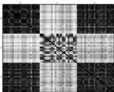
as sticks, and hence usually have a strong variance carried by their first component, followed by a weak second component. On the other hand, the variance of zeros is more equally distributed between the first and second axes. When both weighted sets of points are united, the variance of the mean of both measures has an intermediary behaviour in that respect, and this suffices to discriminate numerically both images. However this strategy fails when using numbers which are not so clearly distinct in shape, or more precisely whose surface cannot be efficiently expressed in terms of Gaussian ellipsoids. To illustrate this we show in Figure 3 the Gram matrix of the linear IGV on 60 images, namely 20 zeros, 20 ones and 20 twos. Though images of ones can be efficiently discriminated from the two other digits, we clearly see that this is not the case between zeros and twos, whose support may seem similar if we try to capture them through Gaussian laws. In practice, the results obtained with the linear IGV on this particular task where so unadapted to the learning goal that the SVM’s trained based on that methodology did not converge in most cases, which is why we discarded it.

8.2 Kernelized IGV

Following previous works (Kondor and Jebara, 2003, Wolf and Shashua, 2003) and as suggested in the initial discussion of Section 5, we use in this section a Gaussian kernel of widthσto incorporate a prior knowledge on the pixels, and equivalently to define the reproducing kernel Hilbert spaceΞ by using

κ((x1,y1),(x2,y2)) =e−

(x1−x2)2+(y1−y2)2

0 1 2

0

1

2

Figure 3: Normalized Gram matrix computed with the linear IGV kernel of twenty images of “0”, “1” and “2” displayed in that order. Darker spots mean values closer to 1, showing that the restriction to “0” and “1” yields good separation results, while “0” and “2” can hardly be discriminated using variance analysis.

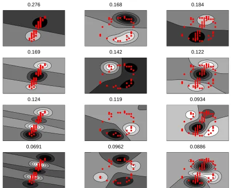
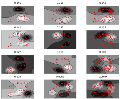
As pointed out by Kondor and Jebara (2003), the pixels are no longer seen as points but rather as functions (Gaussian bells) defined on the components space[0,1]2_{. To illustrate this approach we} show in Figure 4 the first four eigenfunctions of three measures µ1, µ0 and µ1+₂µ0 built from the image of a handwritten “1” and “0” with their corresponding eigenvalues, as well as for images of “2” and “0” in Figure 5.

Settingσ, the width ofκ, to define the functions contained in the RKHSΞis not enough to fully characterize the values taken by the kernelized IGV. We further need to defineη, the regularization parameter, to control the weight assigned to smaller eigenvalues in the spectrum of Gram matrices. Both parameters are strongly related, since the value ofσcontrols the range of the typical eigen-values found in the spectrum of Gram matrices of admissible bases, whereas ηacts as a scaling parameter for those eigenvalues as can be seen in Equation (3). Indeed, using a very smallσvalue, which meansΞis only defined by peaked Gaussian bells around each pixels, yields diagonally dom-inant Gram matrices very close to the identity matrix. The resulting eigenvalues for ˜

K

∆are then all very close to 1_d, the inverse of the amount of considered points. On the contrary, a large value forσyields higher values for the kernel, since all points would be similar to each other and Gram matrices would turn close to the matrix d,dwith a single significant eigenvalue and all others close

to zero. We address these issues and study the robustness of the final output of the k-IGV kernel in terms of classification error by doing preliminary experiments where bothηandσvary freely.

8.3 Experiments on the SVM Generalization Error

0.276 0.168 0.184

0.169 0.142 0.122

0.124 0.119 0.0934

0.0691 0.0962 0.0886

Figure 4: The four first eigenfunctions of respectively three empirical measures µ1 (first column),

0.146 0.168 0.142

0.141 0.142 0.122

0.127 0.119 0.103

0.119 0.0962 0.0949

η_∈10−2_{× {}0.1,0.3,0.5,0.8,1,1.5,2,3,5,8,10,20_}

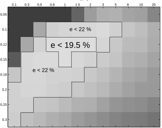
σ_{∈ {}0.05,0.1,0.12,0.15,0.18,0.20,0.25,0.3_}.

For each kernel kη_κ defined by a (σ,η) couple, we trained 10 binary SVM classifiers (each one trained to recognize each digit versus all other digits) on a training fold of our 500 images dataset such that the proportion of each class was kept to be one tenth of the total size of the training set. Using then the test fold, our decision for each submitted image was determined by the highest SVM score proposed by the 10 trained binary SVM’s. To determine train and test points, we led a 3-fold cross validation, namely randomly splitting our total dataset into 3 balanced subsets, using successively 2 subsets for training and the remaining one for testing (that is roughly 332 images for training and 168 for testing). The test error was not only averaged on those cross-validations folds but also on 5 different fold divisions. All the SVM experiments in this experimental section were run using the spider1toolbox. Most results shown here did not improve by choosing different soft margin C parameters, we hence just set C=∞as suggested by default by the authors of the toolbox.

102η

σ

0.1 0.3 0.5 0.8 1 1.5 2 3 5 8 10 20

0.05

0.1

0.12

0.15

0.18

0.2

0.25

0.3

e < 19.5 %

e < 22 %

e < 22 %

Figure 6: Average test error (displayed as a grey level) of different SVM handwritten character recognition experiments using 500 images from the MNIST database (each seen as a set of 25 to 30 randomly selected black pixels), carried out with 3-fold (2 for training, 1 for test) cross validations with 5 repeats, where parametersη(regularization) andσ(width of the Gaussian kernel) have been tuned to different values.

The error rates are graphically displayed in Figure 6 using a grey-scale plot. Note that for this benchmark the best testing errors were reached using aσvalue of 0.12 with anηparameter within 0.008 and 0.02, this error being roughly 19.5%. All values below and on the right side of this zone