Preference Elicitation via Theory Refinement
Peter Haddawy [email protected]
Asian Institute of Technology PO Box 4, Klong Luang Pathumthani 12120, Thailand
Vu Ha [email protected]
Honeywell International 3660 Technology Dr
Minneapolis, MN 55418, USA
Angelo Restificar [email protected]
Department of EE &CS
University of Wisconsin-Milwaukee, PO Box 784 Milwaukee, WI 53201, USA
Benjamin Geisler [email protected]
Department of Computer Science University of Wisconsin-Madison Madison, WI 53706, USA
John Miyamoto [email protected]
Department of Psychology
University of Washington, PO Box 351525 Seattle, WA 98195, USA
Editors: Richard Dybowski, Kathryn Blackmond Laskey, James Myers and Simon Parsons
Abstract
prefer-ences violate a domain theory, and examine the robustness of the KBANN network as this measure of domain theory violation varies.
Keywords: User Modeling, Preference Elicitation, Personalization, Neural Networks, Decision
Theory
1. Introduction
There has been an increasing trend to treat consumers, patients, and computer users as individuals. In medical practice there has been a movement away from the use of general blanket clinical prac-tice guidelines to patient-centered medical care (Gerteis et al., 1993; Couch, 1998; Scott and Lenert, 1998). In e-commerce personalization of products and services has become a recognized way of increasing sales and customer loyalty (Riecken, 2000; Schafer et al., 1999). Companies making ex-tensive use of personalization techniques include Amazon.com, CDnow.com, and Moviefinder.com. Work on the next generation of operating systems is endeavoring to tailor the software to the char-acteristics of the individual user (Horvitz et al., 1998). These applications necessitate the ability to model various aspects of an individual’s attitudes, habits, and behavior, and central among these is the individual’s preferences. Creating a user preference model requires either observing user choice behavior or directly asking questions of the user. In some cases we are forced to ask direct questions since there is no way to observe the choice behavior. In many cases in which we can observe choice behavior, the set of observations may be very small. Thus in modeling user preferences, we are often faced with the problem of creating as accurate a model as possible with as little information as possible.
To reduce the complexity of preference elicitation, traditional approaches from decision analy-sis and multiple criteria decision making make assumptions concerning the structure of preferences (e.g. monotonicity or independence) and then perform elicitation within the constraints of those assumptions. But inaccurate assumptions can result in inaccurate elicitation. Nevertheless, as-sumptions can be a useful guide if they at least approximately apply to some large segment of the population. Ideally we need a method of using assumptions to guide but not constrain the elicitation process. This kind of functionality is provided by theory refinement techniques. The basic idea behind theory refinement is that we can start with a domain theory that may be approximate and incomplete and then correct for inaccuracies and incompleteness by training on examples. If the domain theory is at least approximately correct, we can learn faster with it than without it.
In this paper we explore the use of one particular theory refinement technique, Knowledge-Based Artificial Neural Networks (KBANN), to learn user preferences under conditions of certainty and uncertainty. This is the first theory refinement work that addresses the problem of eliciting user preferences under both certainty and uncertainty. We present a principled approach to applying the KBANN theory refinement technique to preference elicitation by providing general techniques for encoding commonly used assumptions concerning preferences such as preferential independence, monotonicity, dominance, and attitude toward risk. We demonstrate that when such domain knowl-edge is available, even in the form of weak and somewhat inaccurate assumptions, significantly less data is required to build an accurate model of user preferences than when no domain knowledge is provided.
network can be trained to learn fine-grained preference structures from a variety of preferential data, including numeric ratings and simple binary classification. We then empirically compare the KBANN network with a backpropagation artificial neural network (ANN) in terms of learning rate and accuracy. The empirical results show that KBANN outperforms ANN for a number of simulated preference structures.
One hypothesized advantage of the KBANN algorithm is its robustness to noise. According to this hypothesis, the domain theory only needs to be approximately correct for KBANN to be useful. In order to test this hypothesis, we need to define a measure to which a set of preferences violate a domain theory. In a departure from existing syntactic approaches to analyzing domain theory vio-lation, we take a semantic approach to defining such measure, using the notion of similarity among preference structures introduced by Ha and Haddawy (1998). We empirically evaluate the KBANN network and the ANN network in terms of learning rate and accuracy for preferences with varying degrees of domain theory violation. Our empirical findings confirm the robustness hypothesis: the performance of the KBANN network stays quite stable when the preference structures only slightly violate the domain theory.
In Section 3, we explore the KBANN approach to learn user preferences under the presence of uncertainty. We begin by describing a medical experiment, performed by Miyamoto and Eraker (1988), on patients’s preferences regarding survival duration and health quality. The data from this experiment consist of answers to standard-gamble questions. We show how to construct a KBANN network that encodes certain types of dominance relations, can be trained using answers to standard gamble questions, and most importantly, can be used as an approximate representation of a person’s preferences. We empirically compare the KBANN network with a backpropagation network in terms of prediction accuracy and training time, with the KBANN network emerging once again the winner. Section 4 discusses related work and Section 5 presents summary and conclusions.
2. The Certainty Case
In this section, we address the problem of constructing a neural network that represents a user’s preference when there is no uncertainty.
2.1 Modeling User Preferences Using KBANN: A Motivating Example
Suppose we have a user who wishes to find a flight from Milwaukee to Santa Fe. We might describe flights by three attributes: time (t), cost (c), and whether or not the flight has a lay-over (l). Time and cost are continuous, while lay-over is binary. We can assume that the user prefers shorter flights, cheaper flights, and flights without lay-over, all else being equal. Note that this assumption implies, in the language of multi-attribute utility theory (Keeney and Raiffa, 1976), that t, c, and l are each preferentially independent of the other attributes.1 The value of preferential independence lies in the fact that it permits us to represent a high-dimensional value function as a combination of lower dimensional sub-value functions. For example, if we knew in this case that every subset of attributes was preferentially independent of its complement set, then we could represent preferences
1. If the decision outcomes are described in terms of attributes{X1,X2,...,Xn}, attribute X1is said to be preferentially
independent of others if the preference over different values of X1 while holding X2,...,Xn at some fixed level x2,...,xn does not depend on this level. Formally, this means(x1,x2,...,xn)≺(x
0
1,x2,...,xn)⇔(x1,x 0 2,...,x
0
n)≺
over all combinations of t, c, and l as a linear combination of single-attribute value functions. The assumption of preferential independence is generally applicable, but there are certainly exceptions. For example, it is easy to imagine that a traveler normally prefers shorter flights to longer ones, but if there is a lay-over, and the flight is already longer than seventeen hours, then she would prefer a longer lay-over (and thus longer flight) because she could rest more.
We would like to have a user modeling mechanism that can incorporate the preferential inde-pendence of t, c, and l as a domain theory, but can also refine this domain theory based on training examples, some of which may violate the independences. The Knowledge-Based Artificial Neu-ral Network algorithm (Shavlik and Towell, 1989) can provide such mechanism. In a nutshell, the KBANN algorithm initializes a neural network so that it perfectly fits the domain theory, then in-ductively refines this initial hypothesis as needed to fit the training data. The domain theory is a set of non-recursive, propositional Horn clauses. The intuition behind KBANN is that even if the domain theory is only approximately correct, initializing the network to fit this domain theory will give a better starting approximation to the target function than initializing the network to random initial weights.
2.2 Using Artificial Neural Networks to Model User Preferences
We will use the flight selection problem described above as our running example. How should we model user preferences using an ANN? Note that an ANN is in essence just a function that maps a given input to some output. At first, we may be tempted to design an ANN that takes as input the attributes t, c, l of a flight and outputs a numeric rating (or score) for that flight, with a higher rating meaning a more preferred flight. In multi-attribute utility theory, such functions are called value functions. A degenerate case of numeric ratings is binary classification, where items are rated as good or bad, interesting or uninteresting, etc. But numeric ratings, while widely used in modeling preferences in areas such as collaborative filtering, have the disadvantage of fixed granularity: either we choose a coarse granularity and cannot make fine distinctions in preference or we choose a fine granularity and are faced with deciding exactly what rating to assign to an item. For our purpose, the crucial deficiency of numeric ratings is that there appears to be no easy way to encode preferential independences using numeric ratings, i.e., no easy way to initialize an ANN to fit our domain theory of independence assumptions.
An alternative to numeric ratings as a means to represent user preferences is pair-wise compar-ative statements. For example, the user may state that she prefers flight number 1 to flight number 2. Since comparisons are the atoms of preference structures, they are the most general and flexible way to represent preferences. For example, a set of numeric ratings assigned to items can be trans-lated into a set of comparisons among those items: items of higher ratings are more preferred, and items of the same rating are equally preferred. In the followings, we will describe how to construct a KBANN that can be initialized to fit the independence assumptions, can be trained using a wide range of types of data, and can be used to efficiently identify the optimal decision alternative(s).
O := 1 if u(t1,c1,l1)>u(t2,c2,l2) 0 otherwise.
To determine preference or indifference between F1and F2, we examine the value of the output node when the attributes of the two flights are entered as(t1,c1,l1,t2,c2,l2)and(t2,c2,l2,t1,c1,l1). If the output is one and then zero, flight F1is preferred to flight F2; if the output is zero and then one,
F2 is preferred to F1; and if the outputs are zero in both cases the two flights are equally preferred. In the actual implementation, we use target values 0.1 and 0.9 in place of 0 and 1, because of the use of sigmoid functions (Mitchell, 1997).
Next, we will describe the hidden layers of the KBANN. Since a KBANN encodes a domain theory of propositional Horn clauses, we need to express the preferential independences in such clauses:
c1<c2∧t1=t2∧l1=l2 →F1F2
c1=c2∧t1<t2∧l1=l2 →F1F2
c1=c2∧t1=t2∧l1<l2 →F1F2.
Note that formulas such as c1<c2or t1=t2are propositional if considered as atomic formulas, but non-propositional if ci,ti are variables that form part of our logic. We choose to work with the following equivalent set of three clauses instead because they provide more flexibility to the KBANN.2
c1<c2∧t1≤t2∧l1≤l2 →F1F2
c1≤c2∧t1<t2∧l1≤l2 →F1F2
c1≤c2∧t1≤t2∧l1<l2 →F1F2.
Note that in the terminology of multi-attribute utility theory, each clause encodes what is called a dominance relation among the two flights. Since we have three attributes, we have three possible dominance relations, encoded by the three clauses.
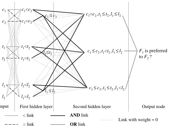
To accommodate this domain theory, we design a KBANN that has two hidden layers (see Fig-ure 1). The first hidden layer is connected to the 6 input nodes. It contains the logic for comparison
<,=,≤between the input nodes(c1,c2),(t1,t2),(l1,l2). The outputs of the first hidden layer are input to the second hidden layer, by means ofAND gates. The nodes of the second hidden layer correspond to the antecedents of the three Horn clauses. The outputs of the second hidden layer are input to the output node by means of anOR gate. Every node at each layer is connected to every node at the next with low randomly chosen weights, except for the case when the link implements a comparison (<,=,≤) or a logical (AND,OR) operator. The detailed implementation of the com-parison and logical operators is described in the Appendix. Note that while it would be possible to compute the comparisons outside the network and include them as separate inputs, represent-ing them as nodes in the network permits them to be modified durrepresent-ing trainrepresent-ing. For example, the
c1<c2
t1≤t2
c1≤c2
t1<t2
l1≤l2
l1<l2
c1<c2,t1≤t2,l1≤l2
c1≤c2,t1<t2,l1≤l2
c1≤c2,t1≤t2,l1<l2 c1
c2
t1
t2
l1
l2
Input First hidden layer Second hidden layer
F1is preferred to F2?
Output node
c1=c2
t1=t2
l1=l2
< link
= link
AND link
OR link
Link with weight≈0
Figure 1: KBANN architecture for modeling user preferences in flights.
user may have a clear preference among two different costs only when they differ by at least some minimal amount. The weights of the network could be modified during training to capture this.
It is easy to see that this KBANN can be trained using a variety of types of data, including numeric ratings, binary classification, or pair-wise comparisons. Also, given a set of n flights, the network can identify the optimal flight(s) using at most 2× n2=n(n−1) forward computations: for each two flights, we determine the preference or indifference between them by inputting their attributes to the KBANN in each of the two orders.
2.3 Empirical Analysis
We experiment with the performance of the KBANN and compare it with the performance of a standard backpropagation artificial neural network (ANN). The ANN has the same input and output units as the KBANN, but has only one single hidden layer. Since ANN learns from data alone, we expect ANN’s performance to be inferior to that of KBANN, given the same number of training instances.
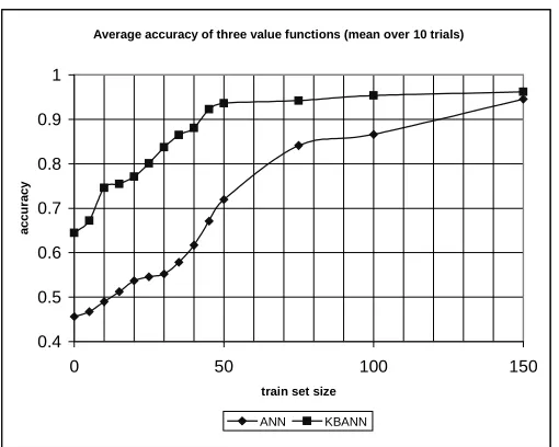
We tested the two networks by randomly generating examples of pair-wise preferences from three different additive value functions: v(t,c,l) =−100t−1c−50l, v(t,c,l) =−50t−1c−100l, and v(t,c,l) =−1t−100c−50l. Note that additive value functions represent preferences consistent with the independence assumptions encoded in the KBANN. Each value function experiment was run 10 times. For each trial we randomly generated a test set of 50 examples different from those used in the training and measured the classification accuracy of the trained network on this set. In order to train and test the network for both possible output values, half the training and testing instances were presented to the network as F1F2and the other half as F1F2.
Average accuracy of three value functions (mean over 10 trials)
0.4 0.5 0.6 0.7 0.8 0.9 1
0 50 100 150
train set size
accu
racy
ANN KBANN
Figure 2: Performance of KBANN and ANN for different TrainSet.
after either 100 epochs or once the activation of the output unit was within 0.25 of correct for 99% of the training instances. The experimental results were averaged over each set of 10 runs. Sim-ilar results were observed for all three value functions. Figure 2 shows the average of the results of the experiments over the three different value functions, with the number of training examples, TrainSize ranging from 0 to 150. The KBANN network consistently outperforms the standard back-propagation network regardless of TrainSize. However, as TrainSize increases, the performance gap between the two networks narrows, and becomes negligible once TrainSize approaches 150. From a different viewpoint, note that KBANN is able to achieve a high accuracy of 84% after only 30 training examples. This level of accuracy is achieved by ANN only after 75 training examples.
2.4 Reducing User Input
0.5 0.6 0.7 0.8 0.9 1
0 5 10 15 20 25
number of flights used
accu
racy
KBANN KBANN w/ bin training
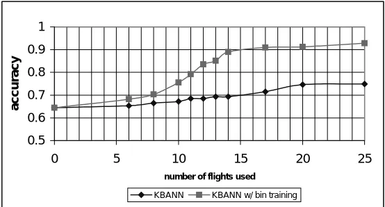
Figure 3: Accuracy of training on examples generated from binary categorization vs those gener-ated randomly, as the total number of flights used in the training examples varies. The used value function is (−1t−100c−50l).
train the KBANN. The results are shown in Figure 3. The KBANN network achieves an accuracy of 89% using only 14 flights - a reduction of 85% (14 versus 60) in the number of flights needed.
2.5 Robustness Analysis
One of the main hypothesized advantages of the KBANN technique is its robustness to noise: the domain theory only needs to be approximately correct for KBANN to be useful. To evaluate this hypothesis in our flight selection domain, we examine the performance of KBANN in learning pref-erences using examples generated from a number of value functions that violate the independence assumptions to various degrees. It is expected that the more a value function violates the domain theory, the worse the performance. The hypothesis is confirmed if this decrease in performance does not occur in a precipitous manner.
2.5.1 DEGREE OFDOMAIN THEORYVIOLATION ANDROBUSTNESSRESULTS
The first issue we have to address in this experiment is to define a measure of domain theory viola-tion. Since we are dealing with domain theory composed of preferential independence assumptions, we will call this measure degree of violating the independences or DOVI. Given a domain theory
D
and a value function u, what would be a good measure VD of u violatingD
? Note that we can viewD
as a set of value functions that satisfyD
. If we have a measureδof distance between two value functions, then we can define a violation measure as the distance between v and the member ofD
that is closest to v:VD(u) =min
KBANN PERFORMANCE
0.6 0.65 0.7 0.75 0.8 0.85 0.9 0.95 1
0 0.2 0.4 0.6 0.8 1
DOVI
Accuracy
KBANN-150 KBANN-100 KBANN-50 KBANN-30
ANN PERFORMANCE
0.6 0.65 0.7 0.75 0.8 0.85 0.9 0.95 1
0 0.2 0.4 0.6 0.8 1
DOVI
Accuracy
ANN-150 ANN-100 ANN-50 ANN-30
Imagine this approach as an analogy to the definition of a distance from a point to a set of points in Euclidean geometry. To define the distanceδbetween two value functions (which represent two preference orders), we use the probabilistic distance, proposed by Ha and Haddawy (1998). This measure is both analytically and computationally tractable for a wide range of representations of preference orders. According to it, the distance between two preference orders is determined by the probability that they disagree in their relative rankings of two randomly chosen outcomes x and y:
δ(f,u) =Pr{((f(x)−f(y))(u(x)−u(y))<0}
Note that if u satisfies
D
, then VD(u) =0. Otherwise, VD(u)will be a number in the interval (0,1].The second issue we have to address is to generate preference orders of varying DOVIs. To this end, we start with some value function u that is consistent with the domain theory
D
. For example, any value function that is a negative linear combination of the attributes t, c, and l is consistent withD
. Subsequently, we permute the orders of k randomly picked outcomes, with different values of k. (We also need to discretize the attributes t and c to make this possible.) It is clear that when k is small, the violation is close to zero, and as we increase k, the perturbed value function is likely to increasingly violate the domain theory.The last issue is the computation of the minimum distance in Equation 1. Since there are ex-ponentially many value functions that satisfy the domain theory
D
, we can only approximate the violation measure by sampling uniformly fromD
. Since the domain theoryD
can be viewed as a partial order on the set of all outcomes(t,c,l), sampling uniformly fromD
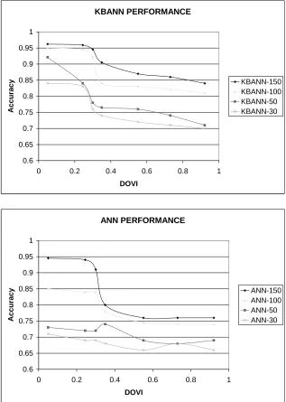
reduces to sampling uniformly from a partial order, which can be done using the same algorithm by Bubley and Dyer (1998) that is used in the Decision Theoretic Video Advisor system (Nguyen and Haddawy, 1999). Figure 4 shows the results of our robustness analysis using seven preference orders with DOVI varying from 0.05 to 0.92. We analyze the performance of KBANN and ANN on these seven preference orders, using a training set size of 30, 50, 100, and 150, and keeping the test set size constant at 50. Notice that for any given number of training examples (30, 50, 100, 150), the performance of KBANN and the ANN decrease as the DOVI increases. KBANN’s performance when the DOVI is 0.24 is still very close to when the DOVI is 0.05. This implies that KBANN is fairly robust to some small amount of noise in the domain theory. The sharpest performance decrease occurs when the DOVI hits the range of 0.3 to 0.35. The fewer examples we use to train the KBANN, the sharper this performance decrease. Fewer training examples means that the KBANN is relying more on the (inaccurate) domain theory. The performance of ANN is dominated in all cases.2.6 Related Work on the Effect of Inaccuracy of Domain Theory
Previous work that examined the effect of inaccuracy of the domain theory on learning performance took a syntactic approach. We now describe two examples of such work to explain the term “syn-tactic”.
to 50 modifications. If the system is trained with 200 examples, the effect on performance of the modifications is fairly negligible.
In their paper describing the KBANN technique, Towell and Shavlik (1994) split domain theory noise into two categories: rule-level noise and antecedent-level noise. Rule-level noise includes missing and added rules, while antecedent-level noise includes missing, extra, and inverted an-tecedents. They start with an initial domain theory for identifying promoter sequences in DNA and probabilistically add each of the four classes of noise to the theory. For each class of noise, they then evaluate the accuracy of the learned concept for a fixed number of examples as the probability of adding noise increases. Although the shapes of the curves for the different classes of noise differ, they are all fairly linear.
The approach used in these two papers was to start with a correct or almost correct domain theory and then to make syntactic changes to it and measure the accuracy of the classification of the learned concept as a function of the number of changes to the domain theory. The obvious problem with this approach is that some syntactic changes can have a much greater effect on the meaning of a domain theory than others. This may be the underlying reason that in the experiments in these two papers, the curves showing classification accuracy versus domain theory accuracy are not all monotonic with respect to the amount of noise added.
In contrast, with the use of degree of violating the independences (DOVI), we take a semantic approach to determining the effect of domain theory imprecision on learning performance. Rather than perturb the domain theory, we fix it and then generate examples from preference structures that increasingly conflict with the domain theory. DOVI captures the degree to which a preference structure violates a set of assumptions in terms of the underlying model of preference, rather than in terms of the structure of the assumptions. This approach works well in our experiment, and we believe that it can be useful in other problem domains involving user preferences, where the domain theory may contain rules that are not preferential independence statements.
3. The Uncertainty Case
In this section, we address the problem of constructing a neural network that represents a user’s preference under the presence of uncertainty. Before discussing the motivating example, we shall provide some background on utility functions and decision making under uncertainty.
3.1 Preliminary: Utility Functions and the Standard-Gamble-Question Technique
In the case of certainty, decision consequences are certain and often called outcomes. We denote the set of all outcomes byΩ. When the decision consequences are uncertain, they are modeled by probability distributions over outcomes and called prospects. We denote the set of all prospects by
S
. The central result of utility theory is a representation theorem that identifies a set of conditions guaranteeing the existence of a function consistent with the preference of a decision maker (von Neumann and Morgenstern, 1944). This theorem states that if the preference order of a decision maker satisfies a few “rational” properties, then there exists a real-valued function, called utility function u :Ω→ℜover outcomes such that for all prospects P1and P2, P1P2⇔ hu,P1i>hu,P2i. Herehu,Pii, the inner product of the utility vector u and the probability vector Pi, is the expected value of utility function u with respect to the distribution Pi:hu,Pii=EPi[u](i=1,2). In addition,The Maximum Expected Utility paradigm lies at the heart of the theory of decision making under risk. This paradigm prescribes that the optimal decision is the one that maximizes expected utility. The main issue in making this paradigm work in practice is the elicitation of a person’s utility function. A wide range of methods and techniques have been invented for the purpose of eliciting utility functions, almost all of which make use of the Standard-Gamble-Question (SGQ) Technique, described below.
Suppose O1,O2∈Ωare two outcomes such that O1≺O2, and 0<p<1. Let(O1,p,O2)denote a gamble in which O1and O2result with probabilities p and 1−p respectively. When p=0.5, we use[O1,O2]as a shorthand for(O1,0.5,O2). Let∼denote indifference. A SGQ is a question that a decision analyst asks a decision maker, and that has one of the two following forms:
(i) For a given p, for which outcome Oceare you indifferent between it and the gamble
(O1,p,O2)? (i.e. Oce∼(O1,p,O2))
(ii) For a given outcome Ocesuch that O1≺Oce≺O2, for what probability 0<p<1
are you indifferent between Oceand the gamble(O1,p,O2)? (i.e. Oce∼(O1,p,O2))
Here “ce” stands for “certainty equivalent”. The decision maker’s answer to this question will specify the following constraint on her utility function u:
pu(O1) + (1−p)u(O2) =u(Oce).
The most commonly used type of SGQ is type (i), with p=.5. We will refer to this type of question as even-chance SGQ, and denote it as ?[O1,O2].
3.2 Predicting Answers to Standard Gamble Questions Using KBANN: A Motivating Example
Miyamoto and Eraker (1988) described a psychology experiment with 27 inpatients at the Ann Ar-bor Veterans Administration Medical Center and the University of Michigan Hospital. The sample included patients aged between 20 and 50 with cancer, heart disease, diabetes, arthritis, and other serious ailments. The subjects were asked standard gamble questions that involve two attributes: duration of survival (y) and health quality (q). This experiment is designed to test whether the subjects’ preferences satisfy a property called “utility independence”. Survival duration is said to be utility independent of health quality provided that for any durations y1, y2, the duration yce that satisfies yce∼[y1,y2]in health state q is the same for any choice of q.3
The significance of utility independence in this experiment is that, together with several intuitive-looking postulates, they imply that the utility function is multiplicative in terms of the two attributes y and q: u(y,q) = f(y)g(q). Each subject was asked to answer 24 even-chance SGQ’s of the form ?[y1,y2]. The health state is fixed at one of two levels, referred to as “current symptoms” (or poor health) and “freedom from current symptoms” (or good health). The survival duration in the SGQ’s ranges from 0 to 24. Furthermore, all subjects confirmed that they prefer longer survival duration in this range, regardless of the health state.
3. The condition yce∼[y1,y2]is a short-hand for(yce,q)∼[(y1,q),(y2,q)], where(y,q)denotes survival of y years in
constant health state q. As Miyamoto and Eraker noted, this form of utility independence is a special case of more
be trained using the answers to the even-chance questions provided by the subject. The input units of this network are y1, y2, yce, and q. There are two output units o1 and o2. The first output unit
o1activates if[y1,y2]≺yce. The second output unit o2activates if[y1,y2]yce. Neither of the two output units activates if[y1,y2]∼yce. The health state is held at q throughout.
It is not immediately clear that a neural network with the above input and output units can be trained using the answers to even-chance questions provided by the subject. Each answer has the form[y1,y2]∼yce and thus can be used to train the network to produce two inactivated output units. But note that because longer survival is preferred to shorter survival, for any y3 such that
y1≺y3≺yce(we call this y3below-ce),[y1,y2]y3, and for any y3such that yce≺y3≺y2(we call this y3above-ce), [y1,y2]≺y3. We thus can train the network to output any possible combination of values using the below-ce and the above-ce values. For example, if the subject provides the following answer:
[0,12]∼4,
then we can train the network using the following examples:
(Below-ce) Inputs: y1=0,y2=12,yce=3→ Outputs: o1=0.1,o2=0.9 (CE) Inputs: y1=0,y2=12,yce=4→ Outputs: o1=0.1,o2=0.1 (Above-ce) Inputs: y1=0,y2=12,yce=5→ Outputs: o1=0.9,o2=0.1
Again, we use the values 0.1 and 0.9 instead of 0 and 1 to represent inactivated and activated states of the output units respectively because of the presence of the sigmoid functions.
Another concern is the question of whether this neural network is adequate as a representation of the subject’s preferences. After all, it is only capable of judging preference between a 50/50 gamble on two survival durations and a certain survival duration, all considered in a fixed health state q. We note however that if the network is trained with enough data so that it accurately judges this kind of preference, it can be used to provide approximate answers to all even-chance SGQ’s. The answers can then be used to compute the subject’s utility function using methods such as utility curve fitting (Raiffa, 1968; Keeney and Raiffa, 1976). So in the end, our network does represent the subject’s preferences. At any given time in the interview process, we can stop asking the subject more SGQ’s, and train the network using the answers we are given so far. This network will be an approximate representation of the subject’s preferences. The more data the network has been trained on, the more accurate this representation will be.
3.3 Adding Domain Theory to the Network
What kind of domain theory can we incorporate into our network that represent the subject’s pref-erences? We are looking for propositional rules where the consequences are either [y1,y2]≺yce,
y1<yce∧y2≤yce → [y1,y2]≺yce y1≤yce∧y2<yce → [y1,y2]≺yce y1>yce∧y2≥yce → [y1,y2]yce
y1≥yce∧y2>yce → [y1,y2]yce
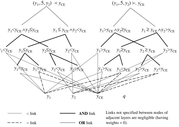
Basically, these rules say that if both outcomes of the even-chance gamble dominate (resp. are dominated by) the certain outcome, then the gamble is preferred to (resp. inferior to) the certain outcome. The KBANN network that incorporates these 4 rules is shown in Figure 5. It has 3 hidden layers, with the first 2 hidden layers implementing the comparisons of survival durations, and the last hidden layer being connected to the 2 output units according to the 4 rules. The implementation of the comparison,AND, andORunits can be found in the Appendix.
Another possible type of prior knowledge, namely attitude toward risk, can also be used as domain theory to construct our KBANN network. In this context, a subject respectively is said to be risk-averse, risk-neutral, or risk-loving if for any survival durations y1and y2, according to her preferences,[y1,y2]≺12(y1+y2),[y1,y2]∼12(y1+y2), or[y1,y2]12(y1+y2), respectively. Thus if we know that a subject is say, risk-loving, we can incorporate the following Horn clauses into our domain theory:
yce≤ y1+y2
2 →[y1,y2]yce.
It is worth mentioning that the above rule supersedes the last two of the four dominance rules, as the antecedents of these two dominance rules are stronger than the risk-loving rule’s.
3.4 Experiment Design and Results
Because in our database of answers to even-chance questions, no assumption about attitude toward risk seems to apply, we perform our experiments with the KBANN constructed from four dominance rules as depicted in Figure 5. For each of the 27 subjects, we run the following experiments. For each x=1,2,...,23, of the 24 answers the subject provided, we leave out x answers for testing purpose and train the network using the remaining 24−x answers. We do this 24 times for each x, taking 24 different combinations of the left-out answers. In the cases when x is 1 or 23, this exhausts all the possible combinations ( 241= 2423=24), while in other cases we take the 24 combinations uniformly randomly from the set of all 24xpossible combinations. For each training/testing answer, we generate 50 below-ce examples ([y1,y2]y3), 50 above-ce examples ([y1,y2]≺y3), in addition to the original example ([y1,y2]∼yce), for a total of 101 examples. The below-ce and the above-ce y3examples are randomly generated from intervals(y1,yce)and(yce,y2)respectively.
We use early stopping with a look-ahead of 100 epochs to avoid overfitting our network. Of all the training examples, we set aside 10% as our validation set. The error function is the standard sum-of-squares-of-errors. Training is stopped if either the current minimum (of the error term of the validation set) does not drop for 100 consecutive epochs, or the total number of epochs has reached 1000.
< link
= link
AND link
OR link
Links not specified between nodes of adjacent layers are negligible (having weights≈0).
y1=yCE
y1 y2 yCE q
y2<yCE y2=yCE
y1<yCE
y1≤yCE y2≤yCE
y1<yCE y2<yCE
y1=yCE y2>yCE y2=yCE
y1>yCE
y1≥yCE y2≥yCE
y1>yCE y2>yCE
y1<yCE∧y2≤yCE y1≤yCE∧y2<yCE y1>yCE∧y2≥yCE y1≥yCE∧y2>yCE (y1,.5, y2)ÿ. yCE
(y1,.5, y2) yCE
Figure 5: KBANN architecture for modeling user preferences in the medical database.
the gamble and the certain outcome is unknown. Ambiguity also results when both output units activate (i.e. have values in the range of[0.8,1]).
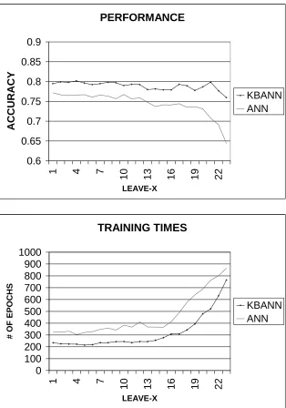
Figure 6 summarizes our main findings. We compare the prediction accuracy and training time of our KBANN network vis-`a-vis a simple backpropagation artificial neural network with the same input and output units and a single hidden layer with 3 hidden nodes. The prediction accuracy and the training time are obtained by averaging over all 27 subjects, and are plotted against LEAVE-X, the number of answers that are left out for testing. KBANN outperforms ANN (i.e. provides better prediction accuracy while requiring less training time) regardless ofLEAVE-X, by up to 10%. As LEAVE-Xincreases, the prediction accuracy shows a decreasing trend (with that of ANN being more pronounced), while the required training time increases. AsLEAVE-X approaches 19, i.e. when we have very few subject answers to train the networks, KBANN outperforms ANN by up to 20%.
In order to judge the statistical significance of our finding, we tested the hypothesis for each
LEAVE-X that the prediction accuracy of KBANN is better than that of ANN. The null hypothesis
is that the difference between the prediction accuracies is zero. Using a right-tail z test, the null hypothesis is rejected with 90% confidence (α=0.1) for 22 out of 23 cases of LEAVE-X, x= 1,2,...,23. In the cases whereLEAVE-Xis at least 19, i.e. when the number of answers available for training is very small (less than 5), the null hypothesis is rejected with 95% confidence (α=0.05). At 87% confidence (α=0.13), all 23 tests rejected the null hypotheses.
4. Related Work
PERFORMANCE
0.6 0.65 0.7 0.75 0.8 0.85 0.9
1 4 7
10 13 16 19 22
LEAVE-X
ACCURACY
KBANN ANN
TRAINING TIMES
0 100 200 300 400 500 600 700 800 900 1000
1 4 7
10 13 16 19 22
LEAVE-X
#
O
F
EPOC
H
S
KBANN ANN
page. The attribute set consists of localized bag-of-words in which words are grouped according to which part of the page they occur in: the title, the page’s URL, etc. The domain theory used by this KBANN consists of user-specified rules such as:
WHEN consecutiveWordsInHypertext (intelligent user interface) STRONGLY SUGGEST FOLLOWING HYPERLINK
This example of a domain theory rule expresses the user’s advice that she is interested in web pages related to intelligent user interfaces. The advice leads to a KBANN in which there is a highly weighted edge between a hidden node and the input node for the string “intelligent user interface” within the WordsInHyperText attribute. The output of this KBANN is the relevance score for the hypertext, contrasted with the present work where the output of our KBANN is a comparison of two alternatives. If the hypertext’s page is fetched, WAWA can analyze it and score it based on its content. Alternatively, the user can score the hypertext’s page. Any difference between these scores and the score predicted by ScoreLink’s KBANN can be used by the backpropagation algorithm to improve ScoreLink. There is no empirical study of WAWA, and no robustness analysis is provided. In an early paper, Wang (1994) discusses the use of ANNs for preference elicitation. He investi-gates two approaches: one in which the output is a utility value and one in which it is an expression of pairwise preference. He discusses the use of ANNs for elicitation of preference under certainty and uncertainty, but the exact network architecture is not shown and the form of the input data the would permit elicitation of prerence under uncertainty is not discussed. Wang shares our concern for flexibility in the representation of preferences: “The commonly used preference models are based on some decomposition rules, whereas the connectionist preference models are ANN-based. This feature relaxes the independence assumptions on the functional form of the preference models and broadens the applicability.” Furthermore, he is also concerned about burdening the user with an excessive number of elicitation questions: “Furthermore, on the DM’s part, more training samples mean more devoted time and effort, and heavier cognitive burden.” But rather than using assump-tions or domain knowledge to reduce the required data, he takes an incremental approach to data collection. His networks are trained with an initial number of training examples. If the desired accuracy on the test set is not reached, then he elicits one more data point and repeats the process. Wang evaluates the accuracy and training time of his ANN on synthetic data from four sample utility functions: additive, multilinear, quadratic, and polynex.
A fairly large number of recommender systems have recently been developed. Below, we sam-ple a few in which there is some degree of combining domain knowledge with data to elicit user preferences. All of these systems fall into the certainty category: they address problems where there is no uncertainty regarding the decision alternatives.
preferences by manipulating a graphical representation of the value function. In contrast with the present work, the additive assumption about user preferences in ATA persists throughout the elic-itation process. Similarly to WAWA (and the vast majority of recommender systems), alternatives (i.e. flights) are not explicitly compared to each other.
Shearin and Lieberman (2001) present Apt Decision, a system that learns user preferences in the domain of rental apartments by obtaining user feedback concerning apartment features. It uses an iterative process of browsing and user feedback. Apt Decision represents user preferences with a value function. It starts with a default model of user preferences in the sense that each feature of an apartment has a base weight determined as part of the domain modeling process. Using an initial profile provided by the user (number of bedrooms, city, price) the system displays a list of sample matching apartments. Weights are changed when the user grabs the feature of an apartment and drags it into a slot on the user profile. The profile contains six positive weight slots: 1 to 6, and six negative weight slots: −1 to−6. Feature weights can also be modified by expressing pair-wise preference among pairs of sample apartments. Profile information is derived by examining the chosen apartment in the context of the current profile. New features are entered into the profile by finding features present in the chosen apartment and not present in other one. An important advantage of the Apt Decision approach is that the user profile is constantly displayed to the user and can be directly modified.
In the case of uncertainty, the only relevant work we are aware of is the work by Chajewska et al. (2000). In this work, Chajewska et al. treat utility as a random variable. They start with a prior probability distribution and then update it based on information elicited from the user. The prior probability can be obtained by analyzing a database of utility functions, when available. The notion of value of information is used to decide on which question to ask next of the user. They evaluate their technique on a database of 51 utility functions elicited from pregnant women considering prenatal testing. Since this approach involves using data to refine prior knowledge, it can also be considered a form of theory refinement. A disadvantage of this approach compared to ours is the difficulty in incorporating intuitive, readily available preferential assumptions such as dominance, monotonicity, and attitude toward risk into the prior probability distribution for the utility random variable.
5. Summary and Conclusions
of certainty, we empirically confirm the robustness of the KBANN approach: even when the domain theory is slightly violated, even when those starting positions are not quite pole positions, KBANN still performs quite close to its best. In the robustness analysis, we define a measure of domain the-ory violation that uses a notion of similarity among preference structures, first introduced by Ha and Haddawy (1998). This semantic definition of the measure of violation is a departure from existing syntactic approaches to analysis of domain theory violation.
The work presented in this paper is only a first step in examining the principled application of theory refinement to preference elicitation and several directions remain open to future research. The KBANN networks we have worked with are propositional representations, which limits the kind of domain theories that can be represented. In some applications we may wish to represent independence assumptions without assuming dominance. This requires using a first-order repre-sentation, quantifying over attribute values. We would then require a technique for refining the first-order domain theory (Richards and Mooney, 1995).
A second limitation of the current work lies in the inability to represent uncertainty in the domain theory. In many domains it is likely that we will have distinct groups of people whose preferences are similar. This idea is well supported by research in market segmentation. Thus, we may wish to work with multiple sets of assumptions, having a probability distribution over them and revising that distribution as we obtain preference data from an individual. Bayesian techniques would be well suited to this problem framework.
Yet another limitation is the scrutability of our representation. In applications such as recom-mendation systems, it can be important to be able to permit the user to examine the current model of her preferences, particularly when the model is being used to filter information. Neural networks are themselves not directly understandable. Towell and Shavlik (1993) have explored techniques for extracting rules from trained KBANN networks, but the techniques do not extract all knowledge contained in the network. One possible approach in our case would be to construct a utility or value function from the network as we have discussed earlier. This could then be presented to the user in graphical or other form.
Finally, we have run experiments in only two domains. Although we don’t expect the perfor-mance of the technique to vary dramatically from one domain to another, it still remains to be seen empirically how the technique will perform in more diverse applications.
Acknowledgments
We thank Jude Shavlik and David Page for helpful discussions and the anonymous reviewers for helpful comments.
Appendix A.
In this Appendix we describe the implementation of the comparison and logical operators. We use sigmoid functions wherever possible to permit the weights to be trained so that the functions can be modified.
f(x,y):= 1 1+e10(x−y)
For the equality (x=y) operator, we set the weights of x and y to 1 and -1 respectively, and use the following sigmoid function:
f(x,y):= 1 1+e20|x−y|−5
The logical operators are implemented in the standard way. For anANDunit (X1∧X2∧...∧Xn→ Y ), all n links Xi→Y are assigned weight w, and the bias on Y is set to(n−12)w. For anOR unit (X1∨X2∨...∨Xn→Y ), all n links Xi→Y are assigned weight w, and the bias on Y is set to 12w. We set w to 4.
References
R. Bubley and M. Dyer. Faster random generation of linear extensions. In Proceedings of the Ninth Annual ACM–SIAM Symposium on Discrete Algorithms, pages 175–186, San Francisco, CA, Jan 1998.
U. Chajewska, D. Koller, and R. Parr. Making rational decisions using adaptive utility elicitation. In Proc AAAI 2000, pages 363–369, July 2000.
J. B. Couch. Disease management: An overview. In J.B. Couch, editor, The Health Care Pro-fessional’s Guide to Disease Management: Patient-Centered Care for the 21st Century. Aspen Publishers, Inc, 1998.
M. Gerteis, S. Edgman-Levitan, and J. Daley. Through the Patient’s Eyes: Understanding and Promoting Patient-Centered Care. Jossey-Bass Health Series, 1993.
V. Ha and P. Haddawy. Towards case-based preference elicitation: Similarity measures on prefer-ence structures. In Proceedings of the Fourteenth Conferprefer-ence on Uncertainty in Artificial Intelli-gence, pages 193–201, July 1998.
E. Horvitz, J. Breese, D. Heckerman, D. Hovel, and K. Rommelse. The lumiere project: Bayesian user modeling for inferring goals and needs of software users. In Proc. Fourteenth Conf. on Uncertainty in AI, pages 256–265, 1998.
R.L. Keeney and H. Raiffa. Decisions with Multiple Objectives: Preferences and Value Tradeoffs. Wiley, New York, 1976.
G. Linden, S. Hanks, and N. Lesh. Interactive assessment of user preference models: The automated travel assistant. User Modeling, June 1997.
T. Mitchell. Machine Learning. McGraw-Hill, 1997.
Conference in Uncertainty In Artificial Intelligence, 1999.
M. Pazzani and Clifford Brunk. Finding accurate frontiers: A knowledge-intensive approach to relational learning. In Proc. AAAI-93, pages 328–334, July 1993.
H. Raiffa. Decision Analysis. Addison-Wesley, Reading,MA, 1968.
Bradley L. Richards and Raymond J. Mooney. Automated refinement of first-order horn-clause domain theories. Machine Learning, 19(2):95–131, 1995.
D. Riecken. Personalized views of personalization. Communications of the ACM, 43(8):26–29, Aug 2000. (Introduction to Special Issue on Personalization).
J.B. Schafer, J. Konstan, and J. Riedl. Recommender systems in e-commerce. In Proc. of the ACM Conference on Electronic Commerce, pages 158–166, 1999.
GC Scott and LA Lenert. Extending contempory decision support designs to patient oriented sys-tems. In Proc. AMIA Annual Fall Symposium, pages 376–380, 1998.
J. Shavlik, S. Calcari, T. Eliasi-Rad, and J. Solock. An instructable, adaptive interface for discover-ing and monitordiscover-ing information on the world wide web. In Proc. IUI-99, 1999.
J. Shavlik and G. Towell. An approach to combining explanation-based and neural learning algo-rithms. Connection Science, 1(3):233–255, 1989.
S. Shearin and H. Lieberman. Intelligent profling by example. In Proceedings of the International Conference on Intelligent User Interfaces (IUI 2001), pages 145–152, Santa Fe, NM, January 2001.
G. Towell and J. Shavlik. Knowledge-based artificial neural networks. Artificial Intelligence, 70 (1-2):119–165, 1994.
Geoffrey G. Towell and Jude W. Shavlik. Extracting refined rules from knowledge-based neural networks. Machine Learning, 13:71–101, 1993.
J. von Neumann and O. Morgenstern. Theory of Games and Economic Behavior. Princeton Uni-vesity Press, 1944.