A Universal Well-Calibrated Algorithm
for On-line Classification
Vladimir Vovk [email protected]
Computer Learning Research Centre Royal Holloway, University of London Egham, Surrey TW20 0EX, UK
Editors: Kristin Bennett and Nicol `o Cesa-Bianchi
Abstract
We study the problem of on-line classification in which the prediction algorithm, for each “sig-nificance level”δ, is required to output as its prediction a range of labels (intuitively, those labels deemed compatible with the available data at the levelδ) rather than just one label; as usual, the examples are assumed to be generated independently from the same probability distribution P. The prediction algorithm is said to be “well-calibrated” for P andδif the long-run relative frequency of errors does not exceedδalmost surely w.r. to P. For well-calibrated algorithms we take the number of “uncertain” predictions (i.e., those containing more than one label) as the principal measure of predictive performance. The main result of this paper is the construction of a prediction algorithm which, for any (unknown) P and anyδ: (a) makes errors independently and with probabilityδat ev-ery trial (in particular, is well-calibrated for P andδ); (b) makes in the long run no more uncertain predictions than any other prediction algorithm that is well-calibrated for P andδ; (c) processes example n in time O(log n).
Keywords: Transductive Confidence Machine, on-line prediction
1. Introduction
Typical machine learning algorithms output a point prediction for the label of an unknown object. This paper continues study of an algorithm called the Transductive Confidence Machine (TCM), introduced by Saunders et al. (1999) and Vovk et al. (1999), that complements its predictions with some measures of confidence. There are different ways of presenting TCM’s output; in this paper (as in the related Vovk, 2002a,b) we use TCM as a “region predictor”, in the sense that it outputs a nested family of prediction regions (indexed by the significance levelδ) rather than a point prediction.
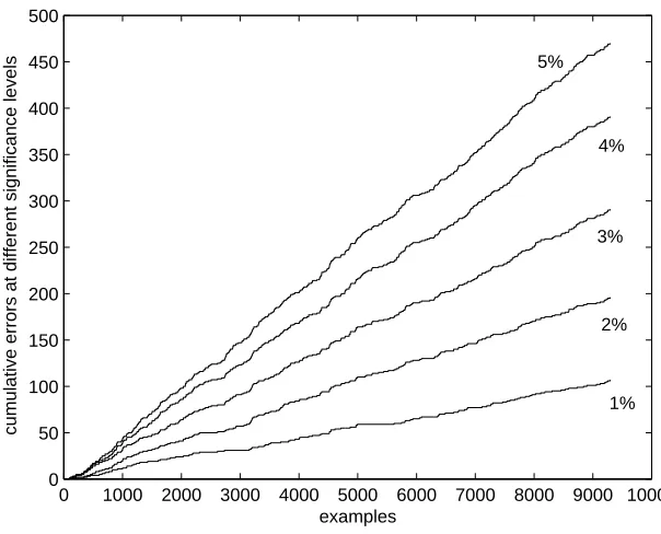
Any TCM is well-calibrated when used in the on-line mode: for any significance level δthe long-run relative frequency of erroneous predictions does not exceedδ. What makes this feature of TCM especially appealing is that it is far from being just an asymptotic phenomenon: a slight modification of TCM called randomized1 TCM (rTCM) makes errors independently at different trials and with probabilityδat each trial. The property of being well-calibrated then immediately follows by the Borel strong law of large numbers. Figure 1 shows the cumulative numbers of errors at the significance levels 1%–5% made on the well-known USPS data set of hand-written digits (randomly permuted); as expected, these are straight lines with the slope approximately equal to the significance level. For proofs and further information, see Vovk (2002a).
0 1000 2000 3000 4000 5000 6000 7000 8000 9000 10000 0
50 100 150 200 250 300 350 400 450 500
examples
cumulative errors at different significance levels
1% 2% 3% 4% 5%
Figure 1: TCM’s cumulative errors at the significance levels 1%–5% on the USPS data set
The justification of the study of TCM given by Vovk (2002a) was its good performance on real-world and standard benchmark data sets. For example, Figure 2 shows that for the significance levels between 1% and 5% most examples in the USPS data set can be predicted categorically (by a simple 1-Nearest Neighbour TCM, used in all experiments reported in this paper): the prediction region contains only one label.
This paper presents theoretical results about TCM’s performance in the problem of classifica-tion, where the number of possible labels is finite; we show that there exists a universal rTCM, which, for any significance levelδand without knowing the true distribution P generating the ex-amples:
• produces, asymptotically, no more uncertain predictions than any other prediction algorithm that is well-calibrated for P andδ;
• produces, asymptotically, at least as many empty predictions as any other prediction algorithm that is well-calibrated for P andδand whose percentage of uncertain predictions is optimal (in the sense of the previous item).
0 1000 2000 3000 4000 5000 6000 7000 8000 9000 10000 0
100 200 300 400 500 600 700 800 900 1000
examples
cumulative uncertain predictions at different significance levels
1%
2%
3%
4%
5%
Figure 2: Cumulative number of “uncertain” predictions (i.e., prediction regions containing more than one label) made by the 1-Nearest Neighbour TCM at the significance levels 1%–5% on the USPS data set
becomes empty does not mean that all potential labels for a new object become equally likely: we should just shift our attention to other significance levels. Figure 3 shows the cumulative numbers of empty predictions for the USPS data set.
The full prediction output by a TCM is a complicated mathematical object: for each significance level δ we have a prediction region. In practice, a good starting point might be first to look at the prediction regions corresponding to two or three conventional significance levels, such as 1% and 5% (afterwards, of course, the prediction regions at other significance levels should be looked at). For example, denotingΓδ the prediction region at significance levelδ, we could say that the prediction is “highly certain” if|Γ1%| ≤1 and “certain” if|Γ5%| ≤1; similarly, we could say that the new object (whose label is being predicted) is “highly atypical” if|Γ1%|=0 and “atypical” if
|Γ5%|=0. In the case of classification, the family of prediction regionsΓδcan be summarized by reporting the confidence
sup{1−δ:|Γδ| ≤1},
the credibility
inf{δ:|Γδ|=0},
and the prediction Γδ, where 1−δ is the confidence (in the case of TCM, |Γδ| ≤1 and usually
0 1000 2000 3000 4000 5000 6000 7000 8000 9000 10000 0
50 100 150 200 250 300
examples
cumulative empty predictions at different significance levels
5%
4%
3%
Figure 3: Cumulative number of empty predictions made by the 1-Nearest Neighbour TCM at the significance levels 1%–5% on the USPS data set (there are no empty predictions for 1% and 2%)
This paper’s result elaborates on Vovk (2002b), where it was shown that an optimal randomized TCM exists when the distribution P generating the examples is known. In the rest of this paper we consider only randomized TCM, so we drop the adjective “randomized”.
The two areas of mainstream machine learning that are most closely connected with this paper are PAC learning theory and Bayesian learning theory. Whereas we often use the rich arsenal of mathematical tools developed in these fields, they do not provide the same kind of guarantees (the right probability of error at each significance level, with errors at different trials independent) under unknown P; for more details, see Vovk (2002a) and references therein. Several papers (such as Rivest and Sloan, 1988; Freund et al., 2004) extend the standard PAC framework by allowing the prediction algorithm to abstain from making a prediction at some trials. Our results show that for any significance levelδthere exists a prediction algorithm that: (a) makes a wrong prediction with relative frequency at most δ; (b) has an optimal frequency of abstentions among the prediction algorithms that satisfy property (a) (for details, see Remark 2 on p. 580). The paper by Freund et al. (2004) is especially close to the approach of this paper, defining a very natural TCM in the situation where a hypothesis class is given (the “empirical log ratio” of Freund et al. (2004), taken with appropriate sign, can be used as an “individual strangeness measure”, as defined in §3).
2. Main Result
called the object space and the labels are elements of a measurable space Y called the label space. In this paper we assume that Y is finite (and endowed with theσ-algebra of all subsets). The protocol includes variables Errδn(the total number of errors made up to and including trial n at significance levelδ) and errδn(the binary variable showing whether an error is made at trial n). It also includes analogous variables Uncδn, uncδn, Empδn, empδnfor uncertain and empty predictions:
Errδ0:=0, Uncδ0:=0, Empδ0:=0 for allδ∈(0,1); FOR n=1,2, . . .:
Reality outputs xn∈X;
Predictor outputsΓδn⊆Y for allδ∈(0,1); Reality outputs yn∈Y;
errδn:= (
1 if yn∈/Γδn
0 otherwise, Err δ
n:=Errδn−1+errδnfor allδ∈(0,1);
uncδn:= (
1 if|Γδn|>1 0 otherwise, Unc
δ
n:=Uncδn−1+uncδnfor allδ∈(0,1);
empδn:= (
1 if|Γδn|=0 0 otherwise , Emp
δ
n:=Empδn−1+empδnfor allδ∈(0,1)
END FOR.
We will use the notation Z :=X×Y for the example space;Γδnwill be called the prediction region (or just prediction).
We will assume that each example zn= (xn,yn), n=1,2, . . ., is output according to a probability
distribution P in Z and the examples are independent of each other (so the sequence z1z2. . . is output by the power distribution P∞). This is Reality’s randomized strategy.
A region predictor is a measurable function
Γδ(x
1,τ1,y1, . . . ,xn−1,τn−1,yn−1,xn,τn), (1)
whereδ∈(0,1), n=1,2, . . ., the(xi,yi)∈Z, i=1, . . . ,n−1, are examples, xn∈X is an object, and
τi∈[0,1](i=1, . . . ,n), which satisfies
Γδ1(x1,τ1,y1, . . . ,x
n−1,τn−1,yn−1,xn,τn)⊆Γδ2(x1,τ1,y1, . . . ,xn−1,τn−1,yn−1,xn,τn)
wheneverδ1≥δ2. The measurability of (1) means that for each n the set n
(δ,x1,τ1,y1, . . . ,xn,τn,yn): yn∈Γδ(x1,τ1,y1, . . . ,xn−1,τn−1,yn−1,xn,τn)
o
⊆(0,1)×(X×[0,1]×Y)n
is measurable.
Since we are interested in prediction with confidence, the region predictor (1) is given an extra input δ∈(0,1), which we call the significance level (typically it is close to 0, standard values being 1% and 5%); the complementary value 1−δis called the confidence level. We will always assume thatτnare independent random variables uniformly distributed in[0,1]. This makes a region
predictor a family (indexed byδ∈(0,1)) of Predictor’s randomized strategies.
is right at trial n and at significance levelδand equal to 1 otherwise. It is always assumed that the random numbersτnused byΓand the random examples znchosen by Reality are independent.
We say that a region predictorΓis (conservatively) well-calibrated for a probability distribution
P in Z and a significance levelδ∈(0,1)if
lim sup
n→∞
Errδn(P∞,Γ)
n ≤δ a.s.
We say (as in Vovk, 2002b) that Γis optimal for P andδif, for any region predictorΓ† which is well-calibrated for P andδ,
lim sup
n→∞
Uncδn(P∞,Γ)
n ≤lim infn→∞
Uncδn(P∞,Γ†)
n a.s. (2)
(It is natural to assume in this and other similar definitions that the random numbers used byΓand
Γ†are independent, but this assumption is not needed for our mathematical results and we do not make it.) Of course, the definition of optimality is natural only for well-calibratedΓ.
A region predictorΓis universal well-calibrated if:
• it is well-calibrated for any P andδ;
• it is optimal for any P andδ;
• for any P, anyδ, and any region predictorΓ†which is well-calibrated and optimal for P and
δ,
lim inf
n→∞
Empδn(P∞,Γ)
n ≥lim supn→∞
Empδn(P∞,Γ†)
n a.s.
Recall that a measurable space X is Borel if it is isomorphic to a measurable subset of the interval[0,1]. The class of Borel spaces is very rich; for example, all Polish spaces (such as finite-dimensional Euclidean spacesRn,R∞, functional spaces C and D) are Borel.
Theorem 1 Suppose the object space X is Borel. There exists a universal well-calibrated region
predictor.
This is the main result of the paper. In §3 we construct a universal well-calibrated region predictor (processing example n in time O(log n)) and in §4 outline the idea of the proof that it indeed satisfies the required properties. Technical details will be given in §5.
3. Construction of a Universal Well-Calibrated Region Predictor
In this section we first define the general notion of Transductive Confidence Machine, and then we specialize it using a nearest neighbours procedure to obtain a universal well-calibrated region predictor.
3.1 Preliminaries
Ifτis a number in[0,1], we split it into two numbersτ0,τ00∈[0,1]as follows: if the binary expansion of τ is 0.a1a2. . . (redefine the binary expansion of 1 to be 0.11. . .), set τ0 :=0.a1a3a5. . . and
τ00:=0.a2a4a6. . .. If τ is distributed uniformly in [0,1], then both τ0 and τ00 are, and they are
independent of each other.
We will often apply our procedures (e.g., the “individual strangeness measure” in §3.2, the Nearest Neighbours rule in §3.3) not to the original objects x∈X but to extended objects(x,σ)∈
˜
X :=X×[0,1], where x is complemented by a random numberσ(to be extracted from one of the
τn). In other words, along with examples(x,y)we will also consider extended examples(x,σ,y)∈
˜
Z :=X×[0,1]×Y.
Let us set X := [0,1]; we can do this without loss of generality since X is Borel. This makes the extended object space ˜X= [0,1]2a linearly ordered set with the lexicographic order:(x1,σ
1)< (x2,σ2)means that either x1=x2andσ1<σ2or x1<x2. We say that(x1,σ1)is nearer to(x3,σ3) than(x2,σ2)is if
|x1−x3,σ1−σ3|<|x2−x3,σ2−σ3|, (3) where
|x,σ|:= (
(x,σ) if(x,σ)≥(0,0)
(−x,−σ) otherwise. (4)
The value |x1−x2,σ1−σ2|plays the role of the distance between extended objects (x1,σ1) and (x2,σ2). Despite such distances being two-dimensional, they are still always comparable using the lexicographic order.
Our construction will be based on the Nearest Neighbours algorithm, which is known to be strongly universally consistent in the traditional theory of pattern recognition (see, e.g., Devroye et al., 1996, Chapter 11); the random componentsσare needed for tie-breaking.
3.2 Transductive Confidence Machines
Transductive Confidence Machine, or TCM, is a way of transition from what we call an “individual strangeness measure” to a region predictor. A family of measurable functions{An: n=1,2, . . .},
where An: ˜Zn→Rn for all n, is called an individual strangeness measure if, for any n=1,2, . . .,
eachαi in
An:(w1, . . . ,wn)7→(α1, . . . ,αn) (5)
is determined by wiand the multiset*w1, . . . ,wn+. (The difference between a multiset*w1, . . . ,wn+
and a set{w1, . . . ,wn}is that the former can contain several copies of the same element.)
The TCM associated with an individual strangeness measure Anis the following region
predic-torΓδ(x1,τ1,y1, . . . ,xn−1,τn−1,yn−1,xn,τn): at any trial n and for any label y∈Y, define
and include y inΓδif and only if
τ00
n<
#{i=1, . . . ,n :αi≥αn} −nδ
#{i=1, . . . ,n :αi=αn}
(6)
(in particular, include y inΓδif #{i=1, . . . ,n :αi>αn}/n>δand do not include y inΓδif #{i=
1, . . . ,n :αi≥αn}/n≤δ).
A TCM is the TCM associated with some individual strangeness measure. It was shown in Vovk (2002a) that
Proposition 2 Every TCM is well-calibrated for every P andδ.
The definition of TCM can be illustrated by the following simple example of an individual strangeness measure, the one used in producing Figures 1–3: mapping (5) can be defined, in the spirit of the 1-Nearest Neighbour Algorithm, as (assuming the objects are vectors in a Euclidean space)
αi:=
minj6=i:yj=yid(xi,xj)
minj6=i:yj6=yid(xi,xj)
,
where d is the Euclidean distance (i.e., an object is considered strange if it is in the middle of objects labelled in a different way and is far from the objects labelled in the same way).
3.3 Universal TCM
Fix a monotonically non-decreasing sequence of integer numbers Kn, n=1,2, . . ., such that
Kn→∞,Kn=o
p
n/ln n (7)
as n→∞. The Nearest Neighbours TCM is defined as follows. Let w1, . . . ,wn be a sequence of
extended examples wi= (xi,σi,yi). To define the correspondingαs , as seen in (5), we first define
Nearest Neighbours approximations Pn6=(y|xi,σi)to the true (but unknown) conditional probabilities
P(y|xi): for every extended example(xi,σi,yi)in the sequence,
Pn6=(y|xi,σi):=N6=(xi,σi,y)/Kn, (8)
where N6=(xi,σi,y)is the number of j=1, . . . ,n such that yj=y and(xj,σj)is one of the Knnearest
neighbours, in the sense of (3), of(xi,σi)in the sequence
((x1,σ1), . . . ,(xi−1,σi−1),(xi+1,σi+1), . . . ,(xn,σn)).
(The upper index 6= reminds us of the fact that (xi,σi) is not counted as one of its own nearest
neighbours in this definition.) If Kn ≥n or Kn ≤0, this definition does not work, so set, e.g.,
Pn6=(y|xi,σi):=1/|Y|for all y and i (this particular convention is not essential since, by (7), 0<
Kn<n from some n on). If the expression “Knnearest neighbours” is not defined because of distance
ties, we again set Pn6=(y|xi,σi):=1/|Y|for all y and i (this convention is not essential since distance
ties happen with probability zero).
Define the “empirical predictability function” fn6=by
fn6=(xi,σi):=max y∈YP
6
=
For each(xi,σi)fix some
ˆ
yn(xi,σi)∈arg max y P
6
=
n (y|xi,σi) (10)
(e.g., take the first element of arg maxyPn6=(y|xi,σi) in a fixed ordering of Y) and define the
map-ping (5) (where wi= (xi,σi,yi), i=1, . . . ,n) setting
αi:=
(
−fn6=(xi,σi) if yi=yˆn(xi,σi)
fn6=(xi,σi) otherwise.
(11)
This completes the definition of the Nearest Neighbours TCM, which will later be shown to be universal.
Proposition 3 Let ∆⊆(0,1) be finite. If X= [0,1]and Kn →∞ sufficiently slowly, the Nearest
Neighbours TCM can be implemented for significance levelsδ∈∆so that the computations at trial n are performed in time O(log n).
Proposition 3 assumes a computational model that allows operations (such as comparison) with real numbers. If X is an arbitrary Borel space, for this proposition to be applicable X should be embedded in[0,1]first; e.g., if X⊆[0,1]n, an x= (x
1, . . . ,xn)∈X can be represented as
(x1,1,x2,1, . . . ,xn,1,x1,2,x2,2, . . . ,xn,2, . . .)∈[0,1],
where 0.xi,1xi,2. . . is the binary expansion of xi. We use the expression “can be implemented” in a
wide sense, only requiring that the implementation should give the correct results almost surely.
4. Fine Details of Region Prediction
In this section we make first steps towards the proof of Theorem 1. Let P be the true distribution in Z generating the examples. We denote by PXthe marginal distribution of P in X (i.e., PX(E):=
P(E×Y)) and by PY|X(y|x)the conditional probability that, for a random example(X,Y)chosen
from P, Y =y provided X =x (we fix arbitrarily a regular version of this conditional probability).
We will often omit lower indicesXandY|Xand P itself from our notation.
The predictability of an object x∈X is
f(x):=max
y∈YP(y|x)
and the predictability distribution function is the function F :[0,1]→[0,1]defined by
F(β):=P{x : f(x)≤β}.
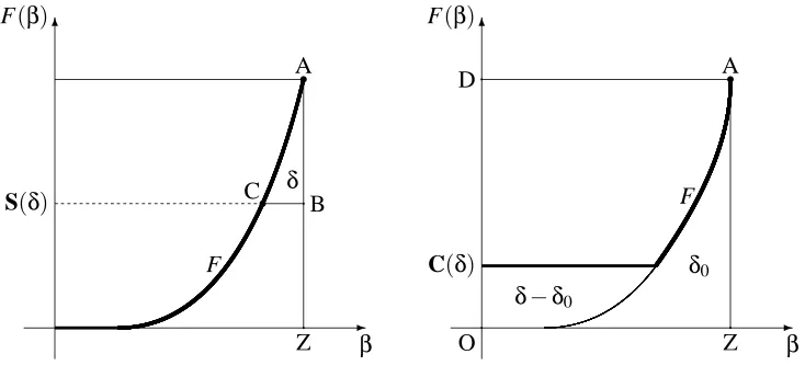
An example of such a function F is given in Figure 4 (left), where the graph of F is the thick line. The success curve SPof P is defined by the equality
SP(δ) =inf
B∈[0,1]:
Z 1
0
(F(β)−B)+dβ≤δ
, (12)
where t+ stands for max(t,0); the function SP is also of the type [0,1]→[0,1]. Geometrically,
-6
β F(β)
r A
pB r C
p Z
δ
S(δ)
F
-6
β F(β)
r A p
D
p Z p
O
δ−δ0
δ0 C(δ)
F
Figure 4: The predictability distribution function F and the success curve S(δ)(left); the comple-mentary success curve C(δ)(right)
move the point B from A to Z until the area of the curvilinear triangle ABC becomesδor B reaches Z; the ordinate of B is then S(δ).
The complementary success curve CPof P is defined by
CP(δ) =sup
B∈[0,1]: B+
Z 1
0
(F(β)−B)+dβ≤δ
, (13)
where sup/0is interpreted as 0. Similarly to the case of S(δ), C(δ)is defined as the value such that the area of the part of the box AZOD below the thick line in Figure 4 (right) isδ(C(δ) =0 if such a value does not exist).
Define the critical significance levelδ0as
δ0:=
Z 1
0
F(β)dβ. (14)
It is clear that
δ≤δ0=⇒
Z 1
0
(F(β)−S(δ))+dβ=δ& C(δ) =0
δ≥δ0=⇒S(δ) =0 & C(δ) +
Z 1
0
(F(β)−C(δ))+dβ=δ.
The following result is proved in Vovk (2002b).
Proposition 4 Let P be a probability distribution in Z andδ∈(0,1) be a significance level. If a region predictorΓis well-calibrated for P andδ, then
lim inf
n→∞
Uncδn(P∞,Γ)
n ≥SP(δ) a.s. (15)
Proposition 5 Let P be a probability distribution in Z andδ∈(0,1) be a significance level. If a region predictorΓis well-calibrated for P andδand satisfies
lim sup
n→∞
Uncδn(P∞,Γ)
n ≤SP(δ) a.s., (16)
then
lim sup
n→∞
Empδn(P∞,Γ)
n ≤CP(δ) a.s.
Theorem 1 immediately follows from Propositions 2, 4, 5 and the following proposition.
Proposition 6 Suppose X is Borel. The Nearest Neighbours TCM constructed in §3.3 satisfies, for
any P and any significance levelδ,
lim sup
n→∞
Uncδn(P∞,Γ)
n ≤SP(δ) a.s. (17)
and
lim inf
n→∞
Empδn(P∞,Γ)
n ≥CP(δ) a.s. (18)
5. Proofs
In this section we will assume that all extended objects (xi,τ0i)∈[0,1]2, where xi are output by
Reality andτi are the random numbers used, are different and that all pairwise distances between
them are also different (this is true with probability one, sinceτ0iare independent random numbers uniformly distributed in[0,1]).
5.1 Proof Sketch of Proposition 3
Without loss of generality we assume that∆contains only one significance levelδ, which will be omitted from our notation. Our computational model has an operation of splittingτ∈[0,1]intoτ0 andτ00(or is allowed to generate bothτ0nandτ00n at every trial n).
We will use two main data structures in our implementation of the Nearest Neighbours TCM:
• a red-black binary search tree;2
• a growing array of nonnegative integers indexed by k∈ {−Kn,−Kn+1, . . . ,Kn}(where n is
the ordinal number of the example being processed).
Immediately after processing the nth extended example(xn,τn,yn)the contents of these data
struc-tures are as follows:
• The search tree contains n vertices, corresponding to the extended examples(xi,τi,yi)seen so
far. The key of vertex i is the extended object(xi,τ0i)∈[0,1]2; the linear order on the keys is
the lexicographic order. The other information contained in vertex i is the random numberτ00i,
the label yi, the set{Pn6=(y|xi,τ0i): y∈Y}of conditional probability estimates (8), the pointer
to the following vertex (i.e., the vertex that has the smallest key greater than(xi,τ0i); if there is
no greater key, the pointer isNIL), and the pointer to the previous vertex (i.e., the vertex that has the greatest key smaller than(xi,τ0i); if(xi,τ0i)is the smallest key, the pointer isNIL).
• The array contains the numbers
N(k):=#{i=1, . . . ,n :αi=k/Kn}
(αiare defined by (11) withσi:=τ0i).
Notice that the information contained in vertex i of the search tree is sufficient to find ˆyn(xi,τ0i)and
αiin time O(1).
We will say that an extended object(xj,τ0j)is in the vicinity of an extended object(xi,τ0i), i6= j,
if there are less than Knextended objects(xk,τ0k)(strictly) between(xi,τ0i)and(xj,τ0j).
When a new object xnbecomes known, the algorithm does the following:
• Generatesτ0nandτ00n.
• Locates the successor and predecessor of(xn,τ0n)in the search tree (using the query SEARCH
and the pointers to the following and previous vertices); this requires time O(log n).
• Computes the estimated conditional probabilities {Pn6=(y|xn,τ0n): y∈ Y}; this also gives
ˆ
yn(xn,τ0n). This involves scanning the vicinity of(xn,τ0n) for the Kn nearest neighbours of
(xn,τ0n), which can be done in time O(Kn): the Kn nearest neighbours can be extracted from
the vicinity of(xn,τ0n)sorted in the order of increasing distances from(xn,τ0n); since initially
the vicinity consists of two sorted lists (to the left and to the right of(xn,τ0n)), the procedure
MERGEused in the merge sort algorithm (see, e.g., Cormen et al. 2001, §2.3.1) will sort the whole vicinity in time O(Kn). Therefore, the required time is O(Kn) =O(log n).
• For each y∈Y looks at what happens if the nth example is(xn,τn,yn) = (xn,τn,y): computes
αn and updates (if necessary)αi for(xi,τ0i)in the vicinity of(xn,τ0n); using the array andτ00n,
finds whether y∈Γn. This requires time O(Kn2) =O(log n), since there are O(Kn)αi’s in the
vicinity of(xn,τ0n)and each of them can be computed in time O(Kn).
• Outputs the prediction regionΓn(time O(1)).
When the label ynarrives, the algorithm:
• Inserts the new vertex (xn,τ0n,τ00n,yn,{Pn6=(y|xn,τ0n): y∈Y}) in the search tree, repairs the
pointers to the following and previous elements for (xn,τ0n)’s left and right neighbours,
ini-tializes the pointers to the following and previous elements for(xn,τ0n)itself, and rebalances
the tree (time O(log n)).
• Updates (if necessary) the conditional probabilities
{Pn6=−1(y|xi,τ0i): y∈Y} 7→ {Pn6=(y|xi,τ0i): y∈Y}
for the 2Kn existing vertices (xi,τ0i) in the vicinity of (xn,τ0n); this requires time O(Kn2) =
• Updates the array, changing N(Knαi) for the(xi,τ0i)= (6 xn,τ0n)in the vicinity of(xn,τ0n)and
for both old and new values ofαi and changing N(Knαn)(time O(Kn) =O(log n)).
In conclusion we discuss how to do the updates required when Knchanges. At the critical trials
n when Kn changes the array and the estimated conditional probabilities Pn6=(y|xi,τ0i) have to be
recomputed, which, if done naively, would require timeΘ(nKn).
The assumption we have made about Kn so far is that Kn=O(√log n). We now also assume
that Knis monotonic non-decreasing and
#{n : Kn<c}=O(#{n : Kn=c}) (19)
as c→∞. This is the full explication of the “Kn→∞sufficiently slowly” in the statement of the
lemma, as used in this proof.
An epoch is defined to be a maximal sequence of ns with the same Kn. Since the changes that
need to be done when a new epoch starts are substantial, they will be spread over the whole pre-ceding epoch; we will only discuss updating the estimated conditional probabilities Pn6=(y|xi,τ0i):
the array is treated similarly. An epoch is odd if the corresponding Kn is odd and even if Kn
is even. At every step in an epoch we prepare the ground for the next epoch. By the end of epoch n=A+1,A+2, . . . ,B we need to change B sets {Pn6=(y|xi,τ0i): y∈Y} in B−A steps
(the duration of the epoch). Therefore, each vertex of the search tree should contain not only
{Pn6=(y|xi,τ0i)} for the current epoch but also{P6
=
n (y|xi,τ0i)}for the next epoch (two structures for
holding{Pn6=(y|xi,τ0i)}will suffice, one for even epochs and one for odd epochs). Our assumptions
of the slow growth of Kn, as seen in 19), imply that B=O(B−A). This means that at each step
O(1)sets{Pn6=(y|xi,τ0i)}for the next epoch should be added. This will take time O(Kn) =O(log n).
As soon as a set{Pn6=(y|xi,τ0i): y∈Y} for the next epoch is added at some trial, both sets (for the
current and next epoch) will have to be updated for each new example.
5.2 Proof Sketch of Proposition 5
The proof of Proposition 5 is similar to (but more complicated than) the proof of Theorems 1 and 1r in Vovk (2002b); this proof sketch can be made rigorous using the Neyman–Pearson lemma, as in Vovk (2002b).
We will use the notations g0left and g0right for the left and right derivatives, respectively, of a function g. The following lemma parallels Lemma 2 in Vovk (2002b), which deals with S(δ).
Lemma 7 The complementary success curve C :[0,1]→[0,1]always satisfies these properties:
1. There is a point δ0 ∈[0,1] (namely, the critical significance level) such that C(δ) =0 for
δ≤δ0and C(δ)is concave forδ≥δ0.
2. C0right(δ0)<∞and C0left(1)≥1; therefore, forδ∈(δ0,1), 1≤C0right(δ)≤C0left(δ)<∞and
the function C(δ)is increasing.
3. C(δ)is continuous atδ=δ0; therefore, it is continuous everywhere in[0,1].
Proof sketch The statement of the lemma follows from the fact that the complementary success curve C can be obtained from the predictability distribution function F using these steps (labelling the horizontal and vertical axes as x and y respectively):
1. Invert F: F1:=F−1. 2. Integrate F1: F2(x):=
Rx
0F1(t)dt.
3. Increase F2: F3(x):=F2(x) +δ0, whereδ0:=
R1
0F(x)dx. 4. Invert F3: F4:=F3−1.
It can be shown that C=F4, if we define g−1(y):=sup{x : g(x)≤y}for non-decreasing g (so that
g−1is continuous on the right).
Complement the protocol of §2 in which Reality plays P∞ and Predictor playsΓwith the fol-lowing variables:
errn:= (P×U)
(x,y,τ): y∈/Γδ(x1,τ1,y1, . . . ,xn−1,τn−1,yn−1,x,τ) ,
uncn:= (PX×U)
(x,τ):|Γδ(x1,τ1,y1, . . . ,xn−1,τn−1,yn−1,x,τ)|>1 , empn:= (PX×U)
(x,τ):|Γδ(x1,τ1,y1, . . . ,xn−1,τn−1,yn−1,x,τ)|=0 ,
δbeing fixed and U standing for the uniform distribution in[0,1], and
Errn:=
n
∑
i=1
erri, Uncn:= n
∑
i=1
unci, Empn:= n
∑
i=1 empi.
By the martingale strong law of large numbers, to prove the proposition it suffices to consider only these “predictable” versions of Errn, Uncn, and Empn: indeed, since Errn−Errn, Uncn−Uncn, and
Empn−Empnare martingales (with increments bounded by 1 in absolute value) with respect to the filtration
F
n, n=0,1, . . ., where eachF
nis generated by(x1,τ1,y1), . . . ,(xn,τn,yn), we havelim
n→∞
Errn−Errn
n =0 a.s.,
lim
n→∞
Uncn−Uncn
n =0 a.s.,
and
lim
n→∞
Empn−Empn
n =0 a.s.
(See, e.g., Shiryaev, 1996, Theorem VII.5.4.)
Without loss of generality we can assume that Predictor’s moveΓn at trial n is{yˆ(xn)}(where
x7→yˆ(x)∈arg maxyP(y|x)is a fixed “choice function”) or the empty set /0or the whole label space
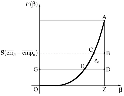
-6
β F(β)
r A
rB r C
rD r
G Er
p Z p
O
εn
S(errn−empn)
Figure 5: An admissible region predictor. The thick line is the predictability distribution function
F; the area of the curvilinear triangle ABC is errn−empn; the area of the rectangle DZOG
is empn; the (non-negative) area of the curvilinear quadrangle BDEC is denotedεn
above the straight line BC in Figure 5,3and that the predictions are empty for the objects below the straight line DG in Figure 5.4 It is clear that for the region predictor to satisfy (16) it must hold that
lim
n→∞
1
n
n
∑
i=1
(εi∧empi) =0
(otherwise Uncncan be decreased substantially, which contradicts (15);εiare defined in the caption
of Figure 5), and so we can assume, without loss of generality, that either εn=0 or empn=0 at
every trial n, i.e., that
uncn=S(errn), empn=C(errn)
at every trial.
Let us check that to achieve (16) the region predictor must satisfy
δ<δ0=⇒lim sup
n→∞
1
n
n
∑
i=1
(erri−δ0)+=0 (20)
δ≥δ0=⇒lim sup
n→∞
1
n
n
∑
i=1
(δ0−erri)+=0, (21)
where the convergence is, as usual, almost certain. It was shown in Vovk (2002b) (Lemma 2) that the success curve S is convex, non-increasing, continuous, and has slope at most−1 before it hits
3. More formally, predictions are certain for new extended objects(x,τ)satisfying
F(x,τ):=F(f(x)−) +τ(F(f(x)+)−F(f(x)−))≥S(errn−empn).
Intuitively, considering extended objects makes the vertical axis “infinitely divisible”.
4. Indeed, predictions of this kind are admissible in the sense that we cannot improve uncnand empnsimultaneously,
and all admissible predictions are equivalent to predictions of this kind. A formal argument for the case where empn
the x axis at δ=δ0. The second implication, (21), now immediately follows from the fact that, underδ≥δ0and (16),
0=lim sup
n→∞
Uncn
n =lim supn→∞
1
n
n
∑
i=1
S(erri)≥lim sup n→∞
1
n
n
∑
i=1
(δ0−erri)+.
The first implication, (20), can be extracted from the chain
Uncn n = 1 n n
∑
i=1 unci=
1
n
n
∑
i=1
S(erri)≥S
1
n
n
∑
i=1 erri
!
=S Errn
n
!
≥S(δ)−ε (22)
(with the last inequality holding almost surely for an arbitraryε>0 from some n on) used by Vovk (2002b, in the proof of Theorems 1 and 1r). Indeed, it can be seen from (22) that, assuming the predictor is well-calibrated and optimal andδ<δ0,
Errn/n→δ a.s.
and, therefore,
S(δ)≥lim sup
n→∞
Uncn
n =lim supn→∞
1
n
n
∑
i=1
S(erri) =lim sup n→∞
1
n
n
∑
i=1
S(erri∧δ0)
≥lim sup
n→∞ S
1
n
n
∑
i=1
(erri∧δ0) !
=lim sup
n→∞ S
Errn n − 1 n n
∑
i=1
(erri−δ0)+ !
=lim sup
n→∞ S δ−
1
n
n
∑
i=1
(erri−δ0)+ !
=S δ−lim sup
n→∞
1
n
n
∑
i=1
(erri−δ0)+ !
almost surely. This proves (20).
Using (20), (21), and the fact that the complementary success curve C is concave, increasing, and (uniformly) continuous forδ≥δ0(see Lemma 7), we obtain: ifδ<δ0,
Empn n = 1 n n
∑
i=1
empi=1
n
n
∑
i=1 C(erri)
≤1 nC
0
right(δ0)
n
∑
i=1
(erri−δ0)+→0 (n→∞); ifδ≥δ0,
Empn n = 1 n n
∑
i=1
C(erri) =
1
n
n
∑
i=1
C(erri∨δ0)
≤C 1
n
n
∑
i=1
(erri∨δ0) !
=C 1
n
n
∑
i=1 erri+
1
n
n
∑
i=1
(δ0−erri)+
!
≤C 1
n
n
∑
i=1 erri
!
+o(1)≤C(δ) +ε,
5.3 Proof Sketch of Proposition 6
Let us first modify and extend the notation Pn6=(y|xi,σi)introduced in (8). Consider the sequence of
extended examples wi= (xi,τ0i,yi), i=1, . . . ,n ((xi,yi)are the first n examples chosen by Reality and
τi are the random numbers used by Predictor). We define the Nearest Neighbours approximations
Pn(y|x,σ)to the conditional probabilities P(y|x)as follows: for every(x,σ,y)∈Z,˜
Pn(y|x,σ):=N(x,σ,y)/Kn, (23)
where N(x,σ,y)is the number of i=1, . . . ,n such that(xi,τ0i)is among the Knnearest neighbours
of(x,σ)and yi=y (this time(xi,τ0i)is not prevented from being counted as one of the Kn nearest
neighbours of(x,σ)if(xi,τ0i) = (x,σ)). We define the empirical predictability function fnby
fn(x,σ):=max
y∈YPn(y|x,σ). (24)
The proof will be based on the following version of a well-known fundamental result.
Lemma 8 Suppose Kn→∞, Kn=o(n), and Y={0,1}. For anyε>0 and large enough n,
P
Z
|P(1|x)−Pn(1|x,σ)|PX(dx)U(dσ)>ε
≤e−nε2/40,
where the outermost probability distributionP(essentially(P×U)∞) generates the extended exam-ples(xi,τi,yi), which determine the empirical distributions Pn.
Proof This is almost a special case of Devroye et al.’s (1994) Theorem 1. There is, however, an important difference between the way we break distance ties and the way Devroye et al. (1994) do this. In that work, instead of our (3),
(|x1−x3|,|σ1−σ3|)<(|x2−x3|,|σ2−σ3|)
is used. (Our way of breaking ties better agrees with the lexicographic order on [0,1]2, which is useful in the proof of Proposition 3 and, less importantly, in the proof of Lemma 10.) It is easy to check that the proof given by Devroye et al. (1994) also works (and becomes simpler) for our way of breaking distance ties.
Lemma 9 Suppose Kn→∞and Kn=o(n). For anyε>0 there exists anε∗>0 such that, for large
enough n,
P
(PX×U)
(x,σ): max
y∈Y|Pn(y|x,σ)−P(y|x)|>ε
>ε
≤e−ε∗n;
in particular,
P(PX×U){(x,σ):|fn(x,σ)−f(x)|>ε}>ε ≤e−ε
∗n
.
Proof We apply Lemma 8 to the binary classification problem obtained from our classification problem by replacing label y∈Y with 1 and replacing all other labels with 0:
P
Z
|P(y|x)−Pn(y|x,σ)|PX(dx)U(dσ)>ε
By Markov’s inequality this implies
P(PX×U){|P(y|x)−Pn(y|x,σ)|>
√ε
}>√ε ≤e−nε2/40, which, in turn, implies
P
(PX×U)
max
y∈Y|P(y|x)−Pn(y|x,σ)|>
√ε
>|Y|√ε
≤e−nε2/40.
This completes the proof, since we can take theεin the last equation arbitrarily small as compared to theεin the statement of the lemma.
We will use the shorthand “∀∞n” for “from some n on”.
Lemma 10 Suppose Kn→∞and Kn=o(n). For anyε>0 there exists anε∗>0 such that, for
large enough n,
P
#ni : maxy
P(y|xi)−P
6
=
n (y|xi,τ0i)
>ε
o
n >ε
≤e−ε∗n.
In particular,
∀∞n :P
# n i :
f(xi)−f
6
=
n (xi,τ0i)
>ε
o
n >ε
≤e−ε∗n.
Proof Since P 6 =
n (y|xi,τ0i)−Pn(y|xi,τ0i)
≤
1
Kn
=o(1),
we can, and will, ignore the upper indices6=in the statement of the lemma. Define
In(x,σ):=
0 if maxy|P(y|x)−Pn(y|x,σ)| ≤ε
1 if maxy|P(y|x)−Pn(y|x,σ)| ≥2ε
(maxy|P(y|x)−Pn(y|x,σ)| −ε)/ε otherwise
(intuitively, In(x,σ)is a “soft version” ofI{maxy|P(y|x)−Pn(y|x,σ)|>ε}).
The main tool in this proof (and several other proofs in this section) will be McDiarmid’s theo-rem (see, e.g., Devroye et al., 1996, Theotheo-rem 9.2). First we check the possibility of its application. If we replace an extended object(xj,τ0j)by another extended object(x∗j,τ∗j), the expression
n
∑
i=1
In(xi,τ0i)
will change as follows:
• the addend In(xi,τ0i)for i= j changes by 1 at most;
• the addends In(xi,τi0)for i6= j such that neither(xj,τ0j)nor(x∗j,τ∗j)are among the Knnearest
• the sum over the at most 4Kn(see below) addends In(xi,τ0i)for i6= j such that either(xj,τ0j)
or(x∗j,τ∗j)(or both) are among the Knnearest neighbours of(xi,τ0i)can change by at most
4Kn 1 ε 1 Kn =4
ε. (25)
The left-hand side of (25) reflects the following facts: the change in Pn(y|xi,τ0i)for i6= j is at most
1/Kn; the number of i6= j such that(xj,τ0j)is among the Kn nearest neighbours of(xi,τ0i)does not
exceed 2Kn (since the extended objects are linearly ordered and (3) is used for breaking distance
ties); analogously, the number of i6= j such that(x∗j,τ∗j) is among the Kn nearest neighbours of
(xi,τ0i)does not exceed 2Kn.
Therefore, by McDiarmid’s theorem,
P ( 1 n n
∑
i=1
In(xi,τ0i)−E
1
n
n
∑
i=1
In(xi,τ0i)
! >ε
)
≤exp−2ε2n/(1+4/ε)2=exp
− 2ε
4 (4+ε)2n
. (26)
Next we find:
E 1n n
∑
i=1
In(xi,τ0i)
!
=E In(xn,τ0n)
≤E In−1(xn,τ0n)
+o(1)
≤E(PX×U){(x,σ): max
y |P(y|x)−Pn−1(y|x,σ)|>ε}+o(1)
≤e−ε∗n+ε+o(1)≤2ε
(the penultimate inequality follows from Lemma 9) from some n on. In combination with (26) this implies
∀∞n :P
( 1
n
n
∑
i=1
In(xi,τ0i)>3ε
)
≤exp
− 2ε
4 (4+ε)2n
,
in particular
P
#{i : maxy|P(y|xi)−Pn(y|xi,τ0i)| ≥2ε}
n >3ε
≤exp
− 2ε
4 (4+ε)2n
.
Replacing 3εbyε, we obtain that, from some n on,
P
#{i : maxy|P(y|xi)−Pn(y|xi,τ0i)|>ε}
n >ε
≤exp
− 2(ε/3)
4 (4+ε/3)2n
,
which completes the proof.
We say that an extended example(xi,τi,yi), i=1, . . . ,n, is n-strange if yi6=yˆn(xi,τ0i); otherwise,
(xi,τi,yi)will be called n-ordinary. We will assume that(fn6=(xi,τ0i),τ00i), i=1, . . . ,n, are all different
-6
β F(β)
r
r
r S(δ)
q
c εεεε
-6
β F(β)
r
r
S(δ) p
p
q
c εεεε
r
Figure 6: Cases F(c) =S(δ)(left) and F(c)>S(δ)(right). The vertical bands of widthεdetermine the division of the first n extended examples into five classes
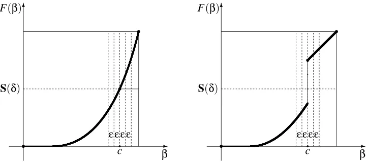
Lemma 11 Suppose (7) is satisfied and δ≤δ0. With probability one, the b(1−S(δ))nc
ex-tended examples with the largest (in the sense of the lexicographic order)(fn6=(xi,τ0i),τ00i) among
(x1,τ1,y1), . . . ,(xn,τn,yn)contain at most nδ+o(n)n-strange extended examples as n→∞.
Proof Define
c :=sup{β: F(β)≤S(δ)}.
It is clear that 0<c<1. Our proof will work both in the case where F(c) =S(δ)and in the case where F(c)>S(δ), as illustrated in Figure 6.
Let ε>0 be a small constant (we will let ε→0 eventually). Define a “threshold”(c0n,c00n)∈ [0,1]2requiring that
Pf(xn) =c,(fn−1(xn,τ0n),τn00)>(c0n,c00n) =F(c)−S(δ)−ε (27)
if F(c)>S(δ); we assume thatεis small enough for
2ε<F(c)−S(δ) (28)
to hold . Among other things this will ensure the validity of the definition (27). If F(c) =S(δ), we set(c0n,c00n):= (c+ε,0); in any case, we will have
Pf(xn) =c,(fn−1(xn,τ0n),τn00)>(c0n,c00n) ≥F(c)−S(δ)−ε. (29)
Let us say that an extended example(xi,τi,yi)is above the threshold if
(fn6=(xi,τ0i),τ00i)>(c0n,c00n);
otherwise, we say it is below the threshold. Divide the first n extended examples (xi,τi,yi), i=
1, . . . ,n, into five classes:
Class II: Those that satisfy f(xi) =c and are below the threshold.
Class III: Those satisfying c−2ε< f(xi)≤c+2εbut not f(xi) =c.
Class IV: Those that satisfy f(xi) =c and are above the threshold.
Class V: Those satisfying f(xi)>c+2ε.
First we explain the general idea of the proof. The threshold(c0,c00)was chosen so that approxi-matelyb(1−S(δ))ncof the available extended examples will be above the threshold. Because of this, the extended examples above the threshold will essentially be theb(1−S(δ))ncextended ex-amples with the largest(fn6=(xi,τ0i),τ00i)referred to in the statement of the lemma. For each of the
five classes we will be interested in the following questions:
• How many extended examples are there in the class?
• How many of those are above the threshold?
• How many of those above the threshold are n-strange?
If the sum of the answers to the last question does not exceed nδby too much, we are done. With this plan in mind, we start the formal proof. (Of course, we will not be following the plan literally: for example, if a class is very small, we do not need to answer the second and third questions.) The first step is to show that
c−ε≤c0n≤c+ε (30)
from some n on; this will ensure that the classes are conveniently separated from each other. We only need to consider the case F(c)>S(δ). The inequality c0n≤c+εfollows from
∀∞n :Pf(xn) =c,fn−1(xn,τ0n)>c+ε <ε<F(c)−S(δ)−ε
Simply combine Lemma 9 with (28). The inequality c−ε≤c0nfollows in a similar way from
∀∞n : Pf(xn) =c,fn−1(xn,τ0n)≥c−ε
=P{f(xn) =c} −P
f(xn) =c,fn−1(xn,τ0n)<c−ε
>F(c)−F(c−)−ε≥F(c)−S(δ)−ε.
Now we are ready to analyze the composition of our five classes. Among the Class I extended examples at most
εn (31)
will be above the threshold from some n on almost surely (by Lemma 10 and the Borel–Cantelli lemma). None of the Class II extended examples will be above the threshold, by definition. The fraction of Class III extended examples among the first n extended examples will tend to
F(c+2ε)−F(c) +F(c−)−F(c−2ε) (32)
To estimate the number NnIV of Class IV extended examples among the first n extended ex-amples, we use McDiarmid’s theorem. If one extended example is replaced by another, NnIV will change by at most 2Kn+1 (since this extended example can affect fn6=(xi,τ0i)for at most 2Knother
extended examples(xi,τi,yi)). Therefore,
P 1 nN IV n − 1
nEN
IV n ≥ε
≤2e−2ε2n/(2Kn+1)2;
the assumption Kn=o
p
n/ln n
and the Borel–Cantelli lemma imply that
1 nN IV n − 1
nEN
IV n <ε
from some n on almost surely. Since
1
nEN
IV
n =P
f(xn) =c,(fn−1(xn,τ0n),τ00n)>(c0n,c00n) ≥F(c)−S(δ)−ε,
as in (29), we have
NnIV>(F(c)−S(δ)−2ε)n (33) from some n on almost surely. Of course, all these examples are above the threshold.
Now we estimate the number NnIV,strof n-strange extended examples of Class IV. Again
McDi-armid’s theorem implies that
1 nN
IV,str
n −
1
nEN
IV,str
n <ε
from some n on almost surely. Now, from some n on,
1
nEN
IV,str
n =P
f(xn) =c,(fn−1(xn,τ0n),τ00n)>(c0n,c00n),yˆn(xn,τ0n)6=yn
=E 1−PY|X yˆn(xn,τ0n)|xn
I{f(xn)=c,(fn−1(xn,τ0n),τ00n)>(c0n,c00n)}
≤e−ε∗n+ε+ (1−c+2ε)
×P{f(xn) =c,(fn−1(xn,τ0n),τ00n)>(c0n,c00n)}
=e−ε∗n+ε+ (1−c+2ε)(F(c)−S(δ)−ε) (34)
≤(F(c)−S(δ))(1−c) +4ε (35)
in the case F(c)>S(δ); the first inequality in this chain follows from Lemma 9: indeed, this lemma implies that, unless an event of the small probability e−ε∗n+εhappens,
P ˆyn(xn,τ0n)|xn
≥Pn−1 yˆn(xn,τ0n)|xn,τ0n
−ε= fn−1 xn,τ0n
−ε≥ f(xn)−2ε. (36)
If F(c) =S(δ), the lines (34) and (35) of that chain have to be changed to
≤e−ε∗n+ε+ (1−c+2ε)P{f(xn) =c,fn−1(xn,τ0n)≥c+ε}
(where the obvious modification of Lemma 9 with all “>ε” changed to “≥ε” is used), but the inequality between the extreme terms of the chain still holds. Therefore, the number of n-strange Class IV extended examples does not exceed
((F(c)−S(δ))(1−c) +5ε)n (37)
from some n on almost surely.
By the Borel strong law of large numbers, the fraction of Class V extended examples among the first n extended examples will tend to
1−F(c+2ε) (38)
as n→∞almost surely. By Lemma 10, the Borel–Cantelli lemma, and (30), almost surely from some n on at least
(1−F(c+2ε)−2ε)n (39)
extended examples in Class V will be above the threshold.
Finally, we estimate the number NnV,str of n-strange extended examples of Class V among the
first n extended examples. By McDiarmid’s theorem,
1
nN
V,str
n −
1
nEN
V,str
n
<ε
from some n on almost surely. Now
1
nEN
V,str
n =P
f(xn)>c+2ε,yˆn(xn,τ0n)6=yn
=E 1−PY|X yˆn(xn,τ0n)|xn
I{f(xn)>c+2ε}
≤e−ε∗n+ε+E (1−f(xn) +2ε)I{f(xn)>c+2ε}
≤e−ε∗n+3ε+E (1−f(xn))I{f(xn)>c+2ε}
=e−ε∗n+3ε+
Z 1
0
(F(β)−F(c+2ε))+dβ
<
Z 1
0
(F(β)−F(c))+dβ+4ε
from some n on. The first inequality follows from Lemma 9, as in (36). Therefore,
1
nN
V,str
n <
Z 1
0
(F(β)−F(c))+dβ+5ε (40)
from some n on almost surely.
Summarizing, we can see that the total number of extended examples above the threshold among the first n extended examples will be at least
(see (33) and (39)) from some n on almost surely. The number of n-strange extended examples among them will not exceed
ε+F(c+2ε)−F(c) +F(c−)−F(c−2ε) +ε
+ (F(c)−S(δ))(1−c) +5ε+
Z 1
0
(F(β)−F(c))+dβ+5ε
n
=
F(c+2ε)−F(c) +F(c−)−F(c−2ε)
+ (F(c)−S(δ))(1−c) +
Z 1
0
(F(β)−F(c))+dβ+12ε
n (42)
(see (31), (32), (37), and (40)) from some n on almost surely. Combining (41) and (42), we can see that the number of n-strange extended examples among theb(1−S(δ))ncextended examples with the largest(fn6=(xi,τ0i),τ00i)does not exceed
F(c+2ε)−F(c) +F(c−)−F(c−2ε) + (F(c)−S(δ))(1−c)
+
Z 1
0
(F(β)−F(c))+dβ+12ε
n+ (F(c+2ε)−F(c) +4ε)n
=
2(F(c+2ε)−F(c)) + (F(c−)−F(c−2ε)) + (F(c)−S(δ))(1−c)
+
Z 1
0
(F(β)−F(c))+dβ+16ε
n
from some n on almost surely. Sinceεcan be arbitrarily small, the coefficient in front of n in the last expression can be made arbitrarily close to
(F(c)−S(δ))(1−c) +
Z 1
0
(F(β)−F(c))+dβ=
Z 1
0
(F(β)−S(δ))+dβ=δ,
which completes the proof.
Lemma 12 Suppose (7) is satisfied. The fraction of n-strange extended examples among the first n
extended examples(xi,τi,yi)approachesδ0asymptotically with probability one.
Proof sketch The lemma is not difficult to prove using McDiarmid’s theorem and the fact that, by Lemma 10, P(yˆn(xi,τi0)|xi)will typically differ little from f(xi). Notice, however, that the part
that we really need in this paper (that the fraction of n-strange extended examples does not exceed
δ0+o(1) as n→∞ with probability one) is just a special case of Lemma 11, corresponding to
δ=δ0.
Lemma 13 Suppose (7) is satisfied and δ>δ0. The fraction of n-ordinary extended examples
among thebC(δ)ncextended examples(xi,τi,yi), i=1, . . . ,n, with the lowest(fn6=(xi,τ0i),τ00i)does