Published online July 23, 2015 (http://www.sciencepublishinggroup.com/j/ajpa) doi: 10.11648/j.ajpa.20150305.11
ISSN: 2330-4286 (Print); ISSN: 2330-4308 (Online)
Analytical Solutions of Undamped and Autonomous
Cubic-Quintic Duffing Equation
Serge Bruno Yamgoué
1, *, Jules Hilaire Kamga
21
Department of Physics, Higher Teacher Training College-Bambili, The University of Bamenda, Bamenda, Cameroon 2
Laboratoire de Mécanique et de Modélisation des Systèmes Physiques (L2MSP), Département de Physique, Université de Dschang, Dschang, Cameroun
Email address:
[email protected] (S. B. Yamgoué), [email protected] (J. H. Kamga)
To cite this article:
Serge Bruno Yamgoué, Jules Hilaire Kamga. Analytical Solutions of Undamped and Autonomous Cubic-Quintic Duffing Equation. American Journal of Physics and Applications. Vol. 3, No. 5, 2015, pp. 159-165. doi: 10.11648/j.ajpa.20150305.11
Abstract:
In this paper, based on a combination of homogenous balance and the rational expansion method, the exact analytical and closed-form solutions of the Duffing equation with cubic and quintic nonlinearities are derived. We focus on heteroclinic and homoclinic solutions which are relevant for the prediction of chaos in forced mechanical systems. The conditions of existence of these solutions which also represent solitons of some wave equations are carefully analyzed.Keywords:
Cubic-Quintic Duffing Equation, Heteroclinic and the Homoclinic Solutions, Soliton1. Introduction
In the description of complex physical processes, simple linear models are often insufficient. Linear effects simply do not fully possess the power to provide a satisfactory description of important processes in optical systems, biological systems, solid state physics, superconducting Josephson arrays, hydrodynamics, and many other subjects. Most real life problems are nonlinear in nature. This has made the study of nonlinear systems which are very complex an important area of study and research. In particular, the traveling wave solutions of nonlinear evolution equations have long been the concern of many mathematicians and physicists [1-5]. Despite the great variety of these nonlinear evolution equations, it is quite interesting to observe that their investigation are very often transformed to that of some universal nonlinear ordinary differential equations by means of appropriate transformations. For instance, the following ordinary differential equation
3 5 0
x+
α
x+β
x +σ
x =ɺɺ (1)
which is a natural generalization of the well known Duffing equation, is commonly encountered in the study of wave phenomena in diverse physical systems. In effect, Aiyong Chen et al transformed the φ6 model to cubic–quintic Duffing oscillator [6], he drawn phase portraits and proved the
monotonicity and critical periods of periodic waves as a function of the wave amplitude. Later Zeid I. A. Al-Muhiameed et al reduced the generalized Zakharov system, the Rangwala and Rao equation and The Chen-Lee-Lin equation to Duffing oscillator [7] and derived the periodic solutions with the aid of the homogenous balance principle. Following this works and in the same spirit Kenmogne and Yemele obtained equation (1) from extended nonlinear Schrodinger equation (ENLS) governing the envelop of modulated waves in a nonlinear discrete electrical transmission line [8]. The associated dynamics was also described in terms of phase portraits.
Besides these wave phenomena, Duffing type equations describe many other kinds of nonlinear oscillatory systems in physics, mechanics and engineering systems such as the classical nonlinear spring system with odd nonlinear restoring characteristics [9], magneto-elastic mechanical systems [10], large amplitude oscillation of centrifugal governor systems [11], nonlinear vibration of beams and plates [12,13] and fluid flow induced vibration [14].
0 = , 0 = 0.
The particular solutions of ordinary differential equations qualified as homoclinic or heteroclinic are also very important in both of wave phenomena and mechanical systems. For wave supporting systems they correspond respectively to the pulse-type and shock or front-type soliton whose importance cannot be overemphasized. Homoclinic and heteroclinic solutions are also central, for example, to the Melnikov theory which is one of the rare analytical theories for predicting the appearance, and hence controlling of chaos in the dynamics of forced mechanical system.
Despite this great importance of homoclinic and heteroclinic solutions there is, to the best of our knowledge, no work which focuses systematically on their analytical expressions for the ubiquituous Duffing equation oscillator (1). It is worth to mention that the knowledge of these exact solutions is also useful for generalizing and/or benchmarking the algorithms to automate the solving of ODEs by computer algebra systems. It is then our purpose in this paper to provide a systematic analysis of these specific types of solutions for this equation. We discuss the conditions of existence and give simple exact and closed-form expressions.
This paper is structured as follows. In section 2 we present the methodology used to derive the solutions. Then the results follow in section 3. And lastly section 4 closes the paper with our conclusion.
2. Methodology
Our concern is the expressions of the solutions of (1) for which the trajectories are asymptotic to at least one unstable equilibrium position of the corresponding physical system. They can be determined as stationary solutions of (1) which correspond to a maximum of the potential.
2 4 6
( )
2 4 6
V x =α x +β x +σ x (2)
These particular trajectories are called separatrixes because they are the boundaries between different types of trajectories in the phase plane: bounded/unbounded or cross-wells / confined-in-wells.
Our methodology for computing the desired analytical solutions is a modified version of one which has been implemented in some softwares for the same purpose [18]. The strategy is to assume the solutions of the ODE in consideration in the form of a polynomial in an auxiliary function f (which may be one of tanh, sech, cosh, sinh, exp and the identity). The degree of this polynomial, m , is determined using the principle of homogenous balance [18]. It consists of requiring that the linear term with the highest order derivative and the highest nonlinear term of the equation balance each other for the monomialf t( )m. In the case of (1) we find thatm=1/ 2. Then we make the change of dependent variable x t( )= y t( ) and obtain
2 2 3 4
2ɺɺyy−yɺ +4αy +4βy +4σy =0 (3)
By repeating the homogenous balance to the new equation, we findm=2. Exact solutions which are polynomials inf , if they exist, must be at most of degree two. Our investigations lead to the conclusion that no such solution exists forσ ≠0. The solutions presented in the next section for this case have been obtained by going beyond polynomial representation, and considering rational forms with numerator and denominator of degree at most two in the auxiliary function f ; with the coefficients to be determined. As usual, each of this so-called “ansatz” is substituted in the differential equation (3). Upon reducing the resulting expression to the same denominator, the numerator can be put in the form of a polynomial in the auxiliary function f . By equating each of its coefficients to zero, one forms a system of nonlinear algebraic equations in the coefficients of the initial ansatz. Exact solutions of this system of algebraic equations, if any, also determine exact solutions of the initial ODE through the assumed ansatz. See [18] and references cited therein for more details. The whole analysis is performed with the help of the MAPLE software.
3. Results
3.1. Cubic Duffing Equation:σ=0
We consider first the now classical case of the cubic Duffing equation which is when σ=0. It is well-known that for it to admit unstable equilibrium, the product of its two coefficients must be less than zero in a strict sense: αβ<0. This condition can be fulfilled in two ways.
3.1.1 Cubic Duffing Equation Associated With Double-Wells Potential: σ =0and β>0 and α<0
When β>0 and α<0in addition to σ=0, the shape of the potential energy function defined in Eq.(2) is a double-wells, as depicted in Fig. 1a. We will use the superscript (s) and (u) to indicate respectively stable and unstable equilibrium; and the subscript l, 0 and r to denotes respectively negative, null and positive equilibrium values. In our figures, we use the notation such as Xr( )u to represents the
point of coordinates xr( )u,V x
( )
r( )u
The expressions of the fixed points and analytical solution of the separatrix for Eq.(1) for σ=0,β>0 and α<0are given by
( )u
r
x α
β −
= , 0( ) 0
u
x = ,xl( )s = −xr( )s , ( )
( )
(
)
2 ssech
ho r
x t = x t −α (4)
“amplitude" A= 2xr( )s of the homoclinic solution xho( )t can be obtained as the solution of the algebraic equation
( ) 0
( ) ( u ) 0
V A −V x = .
Remark: It is easy to verify that if x t( )is a solution of (1) then x(−t) and −x t( ) are also solutions. This implies that other solutions can be obtained by multiplying any of the “amplitude" or the pseudo-frequency ω= −α by −1. To save space, we give only one solution with positive amplitude and frequency.
Figure 1a. A bounded double-well potential: ( , , )α β σ = −( 1,1, 0).
Figure 1b. Profile of homoclinic solution (4) for( , , )α β σ = −( 1,1, 0).
Figure 1c. Phase portrait of homoclinic solution (4) for ( , , )α β σ = −( 1,1, 0).
3.1.2. Cubic Duffing Equation Associated with
Double-Hump Potential: σ=0and β<0 and α>0.
Figure 2a. A double-hump potential: ( , , )α β σ =(1, 1, 0)− .
For σ=0 , β <0 and α >0in addition to σ =0 , the shape of the potential energy function defined in Eq.(2) is a double-hump, as depicted in Fig. 2a. The expressions of the fixed points and analytical solution of the separatrix for Eq.(1) are given in this case by
( )u
r
x α
β =
− , 0( ) 0
u
x = ,xl( )u = −xr( )u , xhe
( )
t =xr( )u tanh(
t α/ 2)
(5)For this case, the separatrix connects
( )
xl( )u ,0 to( )
x( )ru ,0and is qualified as heteroclinic orbit because two distinct unstable equilibrium points are concerned with the connection. It separates bounded, periodic oscillatory motions about
( )
( ) 0 ,0s
x from unbounded non-periodic ones.
3.2. Cubic-Quintic Duffing Equation with Globally Bounded Potential σ>0
After the classical cubic Duffing equation, we turn our attention to the situations where the quintic coefficient is nonzero. We begin the investigation with the case where the potential is bounded globally, i.e., V(±∞ = +∞) . This happens when σ>0.
3.2.1. The Double-Wells Cubic Quintic Duffing Oscillator :
0
σ > and α≤0
The first case of globally bounded cubic-quintic Duffing potential we consider is the one for which this potential looks similar to that portrayed in Fig. 1a. This is the case when
0
α≤ . Under this condition there exist three equilibrium points. Exactly as for the cubic Duffing equation with globally bounded wells, the origin is an unstable fixed point: x( )0u =0;
and two stable ones are located symmetrically on each side of it:
( ) 2 0
4 2 s
x β ασ β
σ
− −
= , xl( )s = −xr( )s (6)
-30 -20 -10 0 10 20 30
0.2 0.4 0.6 0.8 1 1.2 1.4
t
xh
o
(t
)
0.2 0.4 0.6 0.8 1 1.2 1.4 -0.6
-0.4 -0.2 0 0.2 0.4 0.6
xho
x ho
The expression of the homoclinic orbit depends however on whether the linear coefficient α is zero or not.
For strictly negative linear coefficient, α<0 , the homoclinic orbit exists for any real value of the coefficient of the cubic term β . It reads as
( )
(
)
2
1 sinh ho
A
x t
B t α
=
+ − (7)
with
2
9 48 3
1 2
A β ασ β
σ
− −
= ,
2 2
9 48 3 16
8
B β ασ β ασ
ασ
− − +
= (8)
When α =0, the homoclinic orbit still exists but only for
0
β< . Its expression degenerates to an algebraic one according to
( )
6 2 24 ho
x t
t
β σ β
− =
+ (9)
Figure 2b. Analytical heteroclinic solution (5) for ( , , )α β σ = −(1, 1, 0).
Figure 2c. Phase portrait of heteroclinic solution (5) for
( , , )α β σ =(1, 1, 0)− .
3.2.2. The Triple-Wells Cubic-Quintic Duffing Oscillator :
0
σ > , β<0and
2
0 4
β α
σ < <
The potential (2) can possess three wells for some combinations of its coefficients. Namely, for σ >0, β<0
for and
2
0 4
β α
σ
< < the profile of the potential is as depicted in
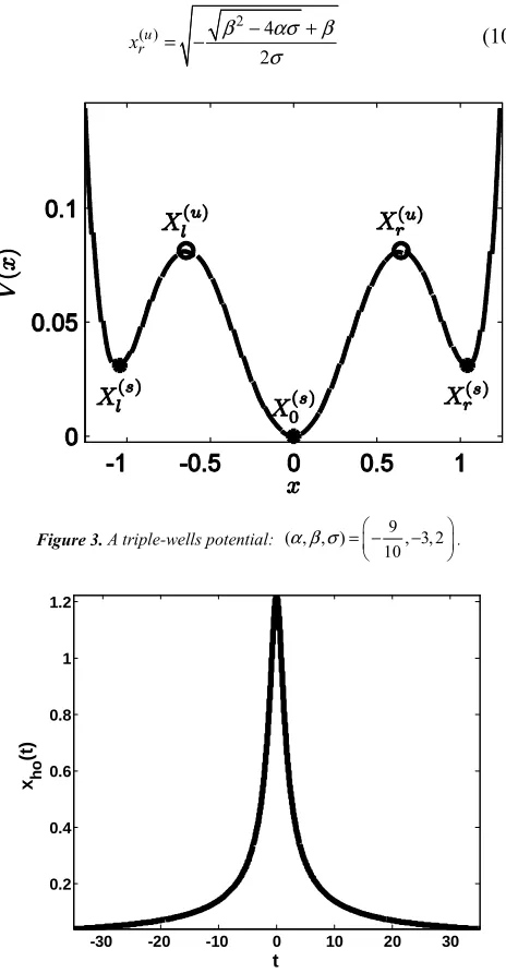
Fig.3. There are five equilibrium positions for the system described by the associated cubic-quintic Duffing oscillator, Eq.(1). These comprise alternately from right to left: a stable fixed point, ( )s
r
x , an unstable fixed point ( )u r
x , the middle
stable fixed point x0( )s =0 together with their symmetric counterparts xl( )u = −xr( )u , and xl( )s = −xr( )s
The expression of ( )s r
x is the same as in Eq.(6) while that
of ( )u r
x is
2
( ) 4
2 u
r
x β ασ β
σ
− +
= − (10)
Figure 3. A triple-wells potential: ( , , ) 9, 3, 2
10
α β σ = − −
.
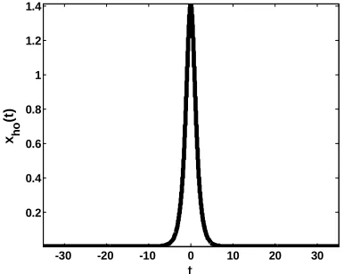
Figure 4a. Analytical homoclinic solution (9) for ( , , ) (0, 1,1)α β σ = − .
-30 -20 -10 0 10 20 30
-1 -0.5 0 0.5 1
t x h
e
(t
)
-1 -0.5 0 0.5 1
0 0.1 0.2 0.3 0.4 0.5 0.6 0.7
x
he x h
e
'
-30 -20 -10 0 10 20 30
0.2 0.4 0.6 0.8 1 1.2
t x h
o
(t
Figure 4b. Phase portrait of homoclinic solution (9) for ( , , )α β σ =(0, 1,1)− .
In this configuration, homoclinic orbits as well as heteroclinic exist simultaneously. The former connect either
of the points
( )
x( )ru ,0 or( )
xl( )u ,0 to itself while the latterconnect these two points to each other. Their expressions are independent of whether V x( 0( )s )>V x( ( )rs ), V x( 0( )s )=V x( r( )s )or
( ) ( ) 0
( s) ( rs)
V x <V x i.e., whether the central wells is less, equally or more deep than the extreme wells respectively. We have
( )
( )
( )
( ) 2
cosh sinh
u r ho
x t
x t
t F
δ δ =
+ (11)
for the homoclinic solution and
( )
( )
( )
( ) 2
sinh cosh
u r he
x t
x t
t F
δ δ =
− (12)
for the heteroclinic solution . In Eqs (11) –(12), is given by Eq.(10) while
2 2
4 4
1 2
ασ β β β ασ δ
σ
− + −
= ,
2 2
2 2
2 4 2
8 4
F
β β β ασ ασ
ασ β β β ασ
+ − −
=
− − −
(13)
3.3. Cubic-Quintic Duffing Equation with Globally Unbounded Potentialσ<0
We consider now the case when the coefficient of the quintic term in Eq.(1) is negative: σ<0. In this case, the potential (2) is globally unbounded, i.e.,. V(±∞ = −∞) .
There are three physically interesting profile considered below.
3.3.1. Existence of Three Unstable Equi-Potential
Equilibrium: σ<0and β>0and
2
3 16
β α
σ =
When the coefficients of Eq.(1) are all nonzero and satisfy
the relationship σ<0and β>0and
2
3 16
β α
σ
= there exists
five equilibrium position, as shown in Fig. 5. Two of these fixed are stable and other unstable. The particularity of the potential here is that all the unstable fixed points are on the same potential level (the same holds for the stable ones). For this case, there are two pairs of heteroclinic orbits.
Figure 5. A potential with three equipotential unstable
equilibrium: ( , , ) 1,1, 3 16
α β σ = − −
Figure 6a. Profile of homoclinic solution (11) for ( , , )α β σ =(0, 1,1)− .
Figure 6b. Phase portrait of homoclinic solution (11) for
( , , )α β σ =(0, 1,1)− .
0.2 0.4 0.6 0.8 1 1.2
-0.4 -0.3 -0.2 -0.1 0 0.1 0.2 0.3 0.4
xho x h
o
'
-30 -20 -10 0 10 20 30
0.4 0.5 0.6 0.7 0.8 0.9 1
t
x h
o
0.4 0.5 0.6 0.7 0.8 0.9 1
-0.2 -0.15 -0.1 -0.05 0 0.05 0.1 0.15 0.2
xho
x h
o
One of the pairs connects Xl( )u to X0( )u . Its analytical expression is
( )
( )
( )
1 exp u r he
x
x t
t
η =
+ (14a)
The other pair connects X0( )u with X0( )u ; its expression is
obtained by replacing ( )u r
x with ( )u r
x
− . Here, ( )u r
x and η are given by
3 2
β η
σ =
−
( ) 1 3
2 u r
x β
σ =
− (14b)
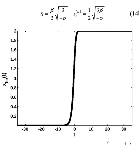
Figure 7. Heteroclinic solution (14a) for ( , , ) 1,1, 3
16
α β σ = − −
.
3.3.2. Other Unbounded Potential Profiles
In each of the last two cases of interest the profile of the potential comprises two wells. On the one hand, if σ<0,
0
β> and
2 2
3
4 16
β α β
σ < < σ the two wells will appear to be
separated by a high potential barrier, as shown in Fig. 8.
Figure 8. A potential with two well separated wells:
3 ( , , ) 1.25,1,
16
α β σ = − −
.
We observe here that the origin is an absolute maximum of the potential. The homoclinic orbits exits and is exactly described by Eqs. (10), (12) and (13). This last configuration is obtained on the other hand for σ<0 , β>0 and
2
3
0 16
β α
σ < < . As one can see from Fig. 9, we may say that the
two wells are embedded in a larger one.
Figure 9. A potential with two well separated wells.
3 ( , , ) 0.875,1,
16
α β σ = − −
.
Then there exist a heteroclinic orbit whose expression is given by Eqs.(10), (12) and (13) and a homoclinic orbit whose expression is given by Eqs.(7)-(8).
4. Conclusion
In this paper the Duffing equation with cubic and quintic nonlinearities which is ubiquitous to the description of many physical systems was considered. We focused on the determination of its solutions that are relevant to the prediction of chaos in forced mechanical systems using the Melnikov theory and which also correspond to solitons solutions of some wave equations. We have achieved this goal by using a combination of homogenous balance and the rational expansion method. Three main classes of solutions including algebraic, exponential and hyperbolic have been obtained and the conditions under which they exist have been unveiled.
References
[1] Camassa, R., Holm, D.: An integrable shallow wave equation with peaked solitons. Phys. Rev. Lett., Vol.71, pp.1661–1664, 1993.
[2] Tian, L., Liang, S.: Global well-posedness and limit behaviorof the solutions to the viscous Degasperis–Procesi equation. J. Math. Phys., Vol.50, 033503, 2009.
[3] Tian, L., Chen, Y., Jiang, X., Xia, L.: Low-regularity solutions of the periodic Fornberg–Whitham equation. J. Math. Phys.,
Vol. 50, 073507, 2009.
-30 -20 -10 0 10 20 30
0.2 0.4 0.6 0.8 1 1.2 1.4 1.6 1.8 2
t x h
e
(t
[4] Cao, C., Geng, X., Wang, H.: Algebro-geometric solution of the (2+1)-dimensional Burgers equation with a discrete variable. J. Math. Phys., Vol.43, pp. 621–643, 2002.
[5] Geng, X., Xue, B.: An extension of integrable Peakon equations with cubic nonlinearity. Nonlinearity, Vol.22, pp.1847–1856 , 2009.
[6] Aiyong Chen · Jibin Li ·Wentao Huang “The monotonicity and critical periods of periodic waves of the φ6 field model” Nonlinear Dyn, Vol.63, pp. 205–215, 2011.
[7] I. A. Zeid Al-Muhiameed and A. B. Emad Abdel-Salam, “Generalized Jacobi Elliptic Function Solution to a Class of Nonlinear Schrödinger-Type Equations”, Mathematical Problems in Engineering, vol. 2011, Article ID 575679, 11 pages, 2011
[8] F. Kenmogne and D. Yemele “Bright and peaklike pulse solitary waves and analogy with modulational instability in an extended nonlinear Schr¨odinger equation” Physical Review E, Vol.88, 043204 , 2013.
[9] A.H. Nayfeh, D.T. Mook, Nonlinear Oscillations, Wiley, New York, 1979.
[10] J. Guckenheimer and P. Holmes, Nonlinear Oscillations, Dynamical Systems and Bifurcations of Vector Fields, Springer-Verlag , 1983.
[11] D.Younesian, H.Askari, Z.Saadatnia, and M. K. Yazdi, ‘‘Periodic solutions for nonlinear oscillation of a centrifugal governor system using the He’s frequency–amplitude formulation and He’s energy balance method’’, Nonlinear Science Letters A, Vol.2, pp. 143–148, 2011.
[12] M.T. Ahmadian, M. Mojahedi, and H. Moeenfard, ‘‘Free vibration analysis of a nonlinear beam using homotopy and modified Lindstedt–Poincare methods’’, Journal of Solid Mechanics, Vol.1, pp. 29–36, 2009. 368 S. Nourazar, A. Mirzabeigy / Scientia Iranica, Transactions B: Mechanical Engineering ,Vol.20, pp 364–368, 2013
[13] F. Bakhtiari-Nejad, and M.Nazari, ‘‘Nonlinear vibration analysis of isotropic cantilever plate with viscoelastic laminate’’, Nonlinear Dynamics, Vol.56, pp. 325–356, 2009. [14] N. Srinil, and H. Zanganeh, ‘‘Modelling of coupled
cross-flow/in-line vortex-induced vibrations using double Duffing and van der Pol oscillators’’, Ocean Engineering, Vol. 53, pp. 83–97, 2012.
[15] S. K. Lai, C. W. Lim, B. S. Wu, C. Wang, C. Q. Zeng, X. F. He: Newton-harmonic balancing approach for accurate solutions to nonlinear cubic-quintic Duffing oscillators. Applied Mathematical Modelling, Vol. 33, pp. 852-866, 2009
[16] Alex Elias-Zuniga: Exact solution of the cubic-quintic Duffing oscillator, Applied Mathematical Modelling, Vol. 37, pp. 2574-2579, 2013
[17] Alex Elias-Zuniga: Solution of the damped cubic-quintic Duffing oscillator by using Jacobi elliptic functions. Applied Mathematics and Computation, Vol. 246, pp. 474-481, 2014 [18] D. Baldwin, Ü. Göktas, W. Hereman, L. Hong, R. S. Martino, J.