Selective Sampling and Active Learning from Single and Multiple
Teachers
Ofer Dekel [email protected]
Microsoft Research One Microsoft Way Redmond, WA, 98052, USA
Claudio Gentile [email protected]
DiSTA, Universit`a dell’Insubria via Mazzini 5
21100 Varese, Italy
Karthik Sridharan [email protected]
Department of Statistics of the Wharton School University of Pennsylvania
3730 Walnut Street
Philadelphia, PA, 19104, USA
Editor:Sanjoy Dasgupta
Abstract
We present a new online learning algorithm in the selective sampling framework, where labels must be actively queried before they are revealed. We prove bounds on the regret of our algorithm and on the number of labels it queries when faced with an adaptive adversarial strategy of generating the instances. Our bounds both generalize and strictly improve over previous bounds in similar settings. Additionally, our selective sampling algorithm can be converted into an efficient statistical active learning algorithm. We extend our algorithm and analysis to the multiple-teacher setting, where the algorithm can choose which subset of teachers to query for each label. Finally, we demonstrate the effectiveness of our techniques on a real-world Internet search problem.
Keywords: online learning, regret, label-efficient, crowdsourcing
1. Introduction
Human-generated labels are expensive. Theactive learningparadigm is built around the idea that we should only acquire labels that actually improve our ability to make accurate predictions.Online selective sampling(Cohn et al., 1990; Freund et al., 1997) is an active learning setting that is mod-eled as a repeated game between alearnerand anadversary. On roundtof the game, the adversary presents the learner with an instancext ∈Rd and the learner responds by predicting a binary label
ˆ
yt∈ {−1,+1}. The learner has access to ateacher,1who knows the correct label for each instance. The learner must now decide whether or not to pay a unit cost and query the teacher for the correct binary labelyt∈ {−1,+1}from the teacher. If the learner decides to issue a query, he observes the correct label and uses it to improve his future predictions. However, when we analyze the accuracy
of the learner’s predictions, we account for all labels, regardless of whether they were observed by the learner or not. The learner has two conflicting goals: to make accurate predictions and to issue a small number of queries.
To motivate the selective sampling setting, consider an Internet search company that uses online learning techniques to construct a (simplified) search engine. In this case, the instancext represents the pairing of a search-engine query with a candidate web page and the task is to predict whether this pair is a good match or a bad match. Clearly, there is no way to manually label the millions of daily search engine queries along with all of their candidate web pages. Instead, an intelligent mechanism of choosing which instances to label is required. Search engine queries arrive in an online manner and a search engine uses its index of the web to match each query with potential candidate URLs, making this problem well suited for the selective sampling problem setting.
The first part of this paper is devoted to the selective sampling framework described above. In Section 2 we present a selective sampling learning algorithm inspired by known ridge regression algorithms (Hoerl and Kennard, 1970; Lai and Wei, 1982; Vovk, 2001; Azoury and Warmuth, 2001; Cesa-Bianchi et al., 2003, 2005a; Li et al., 2008; Strehl and Littman, 2008; Cavallanti et al., 2009; Cesa-Bianchi et al., 2009). To analyze this algorithm, we adopt the model introduced in Cavallanti et al. (2009), Cesa-Bianchi et al. (2009) and Strehl and Littman (2008), where the adversary may choose arbitrary instances, but the teacher is stochastic and samples each label from an instance-dependent distribution. We evaluate the accuracy of the learner using the game-theoretic notion ofregret, which measures the extent to which the learner’s predictions disagree with the teacher’s labels. We prove both an upper bound on the regret and an upper bound on the number of queries issued by the learner.
Our algorithm is an online learning algorithm, designed to incrementally make binary predic-tions on a sequence of adversarially-generated instances. However, we can also convert our algo-rithm into an efficient statistical active learning algoalgo-rithm, which receives a sample of instances from some unknown distribution, queries the teacher for a subset of the labels, and outputs a hy-pothesis with a small risk. The risk of a hyhy-pothesis is its error rate on new instances sampled form the same underlying distribution. We present the details of this conversion in Section 2.5.
In the setting described above, we assumed the learner has access to a single all-knowing teacher. To make things more interesting, we introduce multiple teachers, each with a different area of expertise and a different level of overall competence. On round t, some of the teachers may be experts onxt while others may not be. A teacher who is an expert onxt is likely to provide the correct label, while a teacher who isn’t may give the wrong label. To make this setting as realistic as possible, we assume that the areas of expertise and the overall competence levels of the different teachers are unknown to the learner, and any characterization of a teacher must be inferred from the observed labels.
the assumption that different teachers have different areas of expertise, which allows us to compare each predicted label with the labels provided by experts on the relevant topic.
Recalling the motivating example given above, assume that the Internet search company em-ploys multiple human teachers. Some teachers may be better than others across the board and some teachers may be experts on specific topics, such as sports or politics. Some teachers may know the right answer, while others may think they know the right answers but in fact do not—for this reason we do not rely on the teachers themselves to reveal their expertise regions. For example, say that the search engine receives the web query “nhl new york team” and a candidate url is “kings.nhl.com”; a teacher who is a hockey expert would know that this is a bad match (since New York’s NHL hockey team is called the Rangers and not the Kings) while a non-expert may not know the answer. The learner has no a-priori knowledge of which teacher to query for the label; yet, in our analysis we would like to compare the learner’s prediction to the label given by the expert teacher.
The multiple-teacher selective sampling setting is the focus of the second half of this paper. Specifically, in Section 3 we present a multiple-teacher extension of the (single-teacher) adversarial-stochastic model mentioned earlier, along with two new learning algorithms in this setting. Our model of the teachers’ expertise regions enables our algorithms to gradually identify the expertise region of each teacher. Roughly speaking, the algorithm attempts to measure the consistency of the binary labels provided by each teacher in different regions of the instance space. Our first multiple-teacher algorithm has the property that it either queries all of the multiple-teachers or does not query any teacher, on each round. Our second algorithm is more sophisticated and queries only those teachers it believes to be experts onxt. Again, we provide a theoretical analysis that bounds both regret and number of queries issued to the teachers.
Since our results rely on the specific stochastic model of the teachers, it is natural to question how well this model approximates the real-world. To gain some confidence in our assumptions and in our algorithms, in Section 4 we present a simple empirical study on real data that both validate our theoretical results and demonstrates the effectiveness of our approach.
1.1 Related Work in the Single Teacher Setting
proposed by Hanneke (2009); Koltchinskii (2010) do actually imply estimatingε-minimal sets (or disagreement sets) from empirical data and (local) Rademacher complexities, which makes them computationally hard even for simple function classes, like linear-threshold functions. Finally, pool-based active learning scenarios are considered by Bach (2006) (and the references therein), though the analysis therein is only asymptotic in nature and no quantification is given of the trade-off between risk and number of labels.
To contrast our work with the papers mentioned above, it is worth stressing that our results hold with no stochastic assumption on the source of the instances—in fact, we assume that the instances may be generated by an adaptive adversary. However, as mentioned above, we also show how our online learning algorithm can be converted into a statistical active learning algorithm, with a formal risk bound. Our results in the online selective sampling setting are more in line with the worst-case analyses by Cesa-Bianchi et al. (2006), Strehl and Littman (2008), Cesa-Bianchi et al. (2009) and Orabona and Cesa-Bianchi (2011). These papers present variants of Recursive Least Squares algorithms that operate on arbitrary instance sequences. The analysis by Cesa-Bianchi et al. (2006) is completely worst case: the authors make no assumptions whatsoever on the mechanism generating instances or labels; however, they are unable to prove bounds on the label query rate. The setups by Strehl and Littman (2008), Cesa-Bianchi et al. (2009) and Orabona and Cesa-Bianchi (2011) are closest to ours in that they assume the same stochastic model of the teacher. Our bounds can be shown to be optimal with respect to certain parameters and, unlike competing works on this subject, we are able to face the case when the instance sequencex1,x2, ...is generated by an adaptive adversary, rather than the weakeroblivious adversary, as by, for example, Cesa-Bianchi et al. (2009) and Orabona and Cesa-Bianchi (2011). It is actually this difference that makes it possible the selective sampling-to-active learning conversion. A detailed comparison of our results in the single-teacher setting with the results of the predominant papers on this topic is given in Section 2.6, after our results are presented.
1.2 Related Work in the Multiple Teacher Setting
There is also much related work in the multiple-teacher setting, which is often motivated within recent crowdsourcing applications. We can map the current state-of-the-art on this topic along various interesting axes.
demonstrator to use when teaching a policy to a robot, and Groot et al. (2011) integrate multiple-teacher support into Gaussian process regression learning. Our work in the current paper falls in the second category.
We can also distinguish between algorithms that rely on repeated labeling (where multiple teach-ers label each example), vteach-ersus techniques that assume that each example is labeled only once. Sheng et al. (2008), Snow et al. (2008) and Donmez et al. (2009) collect repeated labels and aggre-gate them (e.g., using a majority vote) to simulate the ground-truth labeling. Some of these papers balance an explore-exploit tradeoff, which determines how many repeated labels are needed for each example. At the opposite end of the spectrum, Dekel and Shamir (2009a) identify low-quality teachers and labels without any repeated labeling. The technique presented in this paper falls in the latter category, since we actively determine which subset of teachers to query on each online round. However, while we do query multiple teachers, we do not assume that the majority vote, or any other aggregate label, is accurate. Still, we do compare to some majority vote of teachers in both our analysis and our experiments.
Next, we distinguish between papers that consider the overall quality score of each teacher (over the entire input space) from papers that assume that each teacher has a specific area of expertise. Most of the papers mentioned above fall in the first category. In the second category, Yan et al. (2010) extend the work in Raykar et al. (2010) (again, maximizing likelihood and using EM) to handle the case where different teachers have knowledge about different parts of the input space. In the present paper, we also model each teacher as an expert on a different subtopic. A closely related research topic is multi-domain adaptation (Mansour et al., 2009a,b), where multiple hypotheses must be optimally combined, under the assumption that each hypothesis makes accurate predictions with respect to a different distribution. Another closely related topic is learning from multiple sources (Crammer et al., 2008), where multiple data sets are sampled from different distributions, and the goal is to optimally combine them with a given target distribution in mind. However, in both of these related problems we are given some prior information on the various distributions, whereas in the multiple-teacher setting we must infer the expertise of each teacher from data.
An interesting variation on the multiple-teacher theme involves allowing each teacher’s quality to vary with time (Donmez et al., 2010).
2. The Single Teacher Case
In this section, we focus on the standard online selective sampling setting, where the learner has to learn an accurate predictor while determining whether or not to query the label of each instance it observes. We formally define the problem setting in Section 2.1 and introduce our algorithm in Section 2.2. We prove upper bounds on the regret and on the number of queries in Section 2.3. We briefly mention how to convert our online learning algorithm into a statistical active learning algorithm in Section 2.4 and Section 2.5, and we compare our results to related work in Section 2.6.
2.1 Preliminaries and Notation
As mentioned above, on round t of the online selective sampling game, the learner receives an instancext ∈Rd, predicts a binary label ˆyt ∈ {−1,+1}, and chooses whether or not to query the correct label yt ∈ {−1,+1}. We setZt =1 if a query is issued on roundt andZt =0 otherwise. The only assumption we make on the process that generatesxt is thatkxtk ≤1; for all we know, instances may be generated by anadaptiveadversary (an adversary that reacts to our previous ac-tions). Note that most of the previous work on this topic makes stronger assumptions on the process that generates xt, resulting in a less powerful setting. As for the labels provided by the teacher, we adopt the standard stochastic linear noise model for this problem (Cesa-Bianchi et al., 2003; Cavallanti et al., 2009; Cesa-Bianchi et al., 2009; Strehl and Littman, 2008) and assume that each yt∈ {−1,+1}is sampled according to the law
P(yt=1|xt) =
1+u⊤xt
2 , (1)
where u∈Rd is a fixed but unknown vector with kuk ≤1. Note that E[yt|xt] =u⊤xt, and we denote this value by∆t. Unlike much of the recent literature on active learning (see Section 1.1), this simple noise model has the advantage of delivering time-efficient algorithms of practical use.
The learner constructs a sequence of linear predictors w0,w1, . . ., where each wt ∈Rd, and predicts ˆyt =sign(∆ˆt)where ˆ∆t =wt−1⊤xt. The desirable outcome is for the sequencew0,w1, . . . to quickly converge tou. LetPt denote the conditional probabilityP(·|x1, . . . ,xt−1,xt,y1, . . . ,yt−1). We evaluate the accuracy of the learner’s predictions using itsregret, defined as
RT = T
∑
t=1
Pt(yt∆ˆt<0)−Pt(yt∆t <0)
.
Additionally, we are interested in the number of queries issued by the learnerNT =∑tT=1Zt. Our goal is to simultaneously bound the regretRT and the number of queriesNT with high probability over the random draw of labels.
Remark 1 At first glance, the linear noise model (1) might seem too restrictive. However, this model can be made implicitly nonlinear by running our algorithm in a Reproducing Kernel Hilbert Space
H
. This entails that the linear operationu⊤xtin (1) is replaced by h(xt), for some (typically nonlinear) function h∈H
. See also the comments at the end of Section 2.2, and those surrounding2.2 Algorithm
The single teacher algorithm is a margin-based selective sampling procedure. The algorithm “Se-lective Sampler” (Algorithm 1) depends on a confidence parameter δ∈(0,1]. As in known on-line ridge-regression-like algorithms (Hoerl and Kennard, 1970; Vovk, 2001; Azoury and War-muth, 2001; Cesa-Bianchi et al., 2003, 2005a; Li et al., 2008; Strehl and Littman, 2008; Cavallanti et al., 2009; Cesa-Bianchi et al., 2009), our algorithm maintains a weight vectorwt (initialized as
w0=0) and a data correlation matrixAt (initialized asA0=I). After receivingxt and predicting ˆ
yt=sign(∆ˆt), the algorithm computes an adaptive data-dependent thresholdθt, defined as
θ2
t = xt⊤At−−11xt
1+4 t−1
∑
i=1
Ziri+36 log t
δ
,
whereri=x⊤i A−i 1xi. The definition ofθt follows from our analysis, and can be interpreted as the algorithm’s uncertainty in its own predictions. More precisely, the learner believes that|∆ˆt−∆t| ≤ θt. A query is issued only if|∆ˆt| ≤θt, or in other words, when the algorithm is unsure about the sign of∆t. In Algorithm 1, this is denoted byZt =11
ˆ
∆2
t ≤θt2}, where 11
· denotes the indicator function.
If the label is not queried, (Zt =0) then the algorithm does not update its internal state (andxt is discarded). If the label is queried (Zt =1), then the algorithm computes the intermediate vector
w′t−1in such a way that ˆ∆′t=wt′−1⊤xt is at most one in magnitude. Observe that ˆ∆t and ˆ∆′t have the same sign and only their magnitudes can differ. In particular, it holds that
ˆ ∆′t=
(
sgn(∆ˆt) if|∆ˆt|>1 ˆ
∆t otherwise .
Next, the algorithm defines the new vectorwt so thatAtwt undergoes an additive update, whereAt is a rank-one adjustment ofAt−1.
The algorithm can be run both in primal form (as in the pseudocode in Algorithm 1) and in dual form (i.e., in a Reproducing Kernel Hilbert Space). It is not hard to show that the algorithm has a quadratic running time per round, where quadratic meansO(d2)if it is run in primal form, and O(Nt2)if it is run in dual form, whereNt=∑i≤tZiis the number of labels requested by the algorithm up to timet. In the dual case, since the algorithm updates only whenZt=1, the number of labels Nt also corresponds to the number of support vectors used to define the current hypothesis.
2.3 Analysis
Ifxt lies along the directions spanned by the previous instances, we show thatxt⊤At−−11xt tends to shrink as 1/Nt. As a result,θt is on the order of log(t/δ)/Nt, andNt only needs to grow at a slow logarithmic rate. On the other hand, if the adversary choosesxt outside of the subspace spanned by the previous examples, then the termx⊤t A−t−11xt causesθt to be large, and the algorithm becomes more likely to issue a query. Overall, to ensure a small value ofθt across the instance space spanned by thext produced by the adversary, the algorithm must queryO log(t)
labels in each direction of this instance space.
As noted above, the adversary can arbitrarily inflate our regret by choosing instances that induce small values of∆t. Recall that a small value of∆timplies that the teacher guesses the labelytalmost at random. Following Cesa-Bianchi et al. (2009), the bounds we prove depend on how many of the instancesxt are chosen such that∆t is very small. Formally, for anyε>0, define
Tε=
T
∑
t=1 1
1{|∆t| ≤ε}. (2)
The following theorem is the main result of this section, and is stated so as to emphasize both the data-dependent and the time-dependent aspects of our bounds.
Theorem 2 Assume that Selective Sampler is run with confidence parameterδ∈(0,1]. Then with probability at least1−δit holds that for all T≥3
RT ≤ inf
ε>0
n
εTε+
2+8 log|AT|+144 log(T/δ) ε
o
=inf
ε>0
n
εTε+O
dlogT+log(T/δ)
ε
o
NT ≤ inf
ε>0
n
Tε+O
log|AT|log(T/δ) +log2 |AT| ε2
o
=inf
ε>0
n
Tε+O
d2log2(T/δ) ε2
o ,
where|AT|is the determinant of the matrix AT.
Note that the bounds above depend ond the dimension of the instance space. In the case of a (possibly infinite-dimensional) Reproducing Kernel Hilbert Space,d is replaced by a quantity that depends on the spectrum of the data’s Gram matrix.
The proof of Theorem 2 splits into a series of lemmas. For everyT >0 andε>0, we define
UT,ε=
T
∑
t=1 ¯ Zt11
∆t∆ˆt<0,∆2 t >ε2 , QT,ε=
T
∑
t=1 Zt11
∆t∆ˆt<0,∆2t >ε2 |∆t|,
where ¯Zt =1−Zt. In the above, UT,ε deals with rounds where the algorithm does not make a
query, whileQT,ε deals with rounds where the algorithm does make a query. The proof exploits
the potential-based method for online ridge-regression-like algorithms we learned from Azoury and Warmuth (2001). See also the works of Hazan et al. (2007), Dani et al. (2008) and Crammer and Gentile (2011) for a similar use in different contexts. The potential function we use is the (quadratic) Bregman divergencedt(u,w) = 12(u−w)⊤At(u−w), whereAt is the matrix computed by Selective Sampler at timet.
The proof structure is as follows. First, Lemma 3 below decomposes the regret RT into three parts:
Algorithm 1:Selective Sampler
input confidence levelδ∈(0,1]
initializew0=0, A0=I fort=1,2, . . .
receive xt ∈Rd:||xt|| ≤1, and set ˆ∆t =wt−1⊤xt
predict yˆt =sgn(∆ˆt)∈ {−1,+1} θ2
t =x⊤t A−t−11xt
1+4∑ti−=11Ziri+36log(t/δ)
Zt =11
ˆ
∆2
t ≤θ2t ∈ {0,1} ifZt =1
query yt∈ {−1,+1}
wt′−1=
wt−1−sgn(∆ˆt)
|∆ˆt|−1
x⊤t A−t−11xt
At−−11xt if|∆ˆt|>1
wt−1 otherwise
At =At−1+xtxt⊤, rt=x⊤t A−t 1xt, wt=A−t 1(At−1wt′−1+ytxt) else
At =At−1, wt=wt−1, rt=0
The bound onUT,ε is given by Lemma 4. For the bound on QT,ε and the bound on the number
of queriesNT, we use Lemmas 5 and 6, respectively. However, both of these lemmas require that
(∆t−∆ˆt)2≤θ2
t for allt. This assumption is taken care of by the subsequent Lemma 7. Sinceεis a positive free parameter, we can take the infimum overε>0 to get the required results. In turn, many of these lemmas rely on technical lemmas given in Appendix A and Appendix B.
Lemma 3 For anyε>0it holds that RT≤εTε +UT,ε + QT,ε.
Proof We have
Pt(∆ˆtyt<0)−Pt(∆tyt <0)
≤ 11∆ˆt∆t ≤0 2Pt(yt=1)−1
= 11∆ˆt∆t ≤0 |∆t|
= 11∆t∆ˆt <0,∆t2≤ε2 |∆t|+11∆t∆ˆt <0,∆t2>ε2 |∆t|
≤ε11∆t∆ˆt <0,∆t2≤ε2 +11∆t∆ˆt<0,∆2t >ε2 |∆t| (3)
=ε11∆t∆ˆt <0,∆2
t ≤ε2 +11
∆t∆ˆt<0,∆2
t >ε2,Zt=0 |∆t|
+11∆t∆ˆt<0,∆2
t >ε2,Zt =1 |∆t|
≤ε11∆t∆ˆt <0,∆t2≤ε2 +Z¯t11∆t∆ˆt <0,∆2t >ε2 (4)
+Zt11
∆t∆ˆt<0,∆2t >ε2 |∆t|.
Lemma 4 For anyε>0and T ≥3, with probability at least1−δ, it holds that
QT,ε ≤
2+8 log|AT|+144 log(T/δ)
ε = O
dlogT+log(T/δ)
ε
.
Proof We begin with
QT,ε =
T
∑
t=1 Zt11
∆t∆ˆt <0 11∆2t >ε2 |∆t|
≤ 1ε T
∑
t=1 Zt11
ˆ
∆t∆t <0 ∆2 t
= 1
ε T
∑
t=1 Zt11
ˆ
∆′t∆t <0 ∆2t .
ˆ
∆′t∆t <0 implies that∆2
t ≤(∆t−∆ˆ′t)2, and therefore the above can be upper bounded by 1
ε T
∑
t=1
Zt(∆t−∆ˆ′t)2.
Next we rely on some standard technical results that are given in the appendix. Lemma 23 (i) upper bounds the above by
2 ε
T
∑
t=1
Zt (yt−∆ˆ′t)2−(yt−∆t)2
+144
ε log(T/δ).
Lemma 25 (iv) further bounds this term by
4 ε
T
∑
t=1 Zt
dt−1(u,wt′−1)−dt(u,wt′) +2 log | At| |At−1|
+144
ε log(T/δ).
After telescoping and using the facts thatd0(u,w′0) =d0(u,w0) =||u||2/2≤1/2 and|A0|=1, the above is bounded by
2+8 log|AT|+144 log(T/δ)
ε ,
which is in factO
dlogT+log(T/δ)
ε
in the finite-dimensional case. This concludes the proof.
Lemma 5 Assume that(∆t−∆ˆt)2≤θ2
t holds for all t. Then, for anyε>0, we have UT,ε=0
Proof We rewrite our assumption(∆t−∆ˆt)2≤θ2 t as
∆t∆ˆt≥∆ˆ 2
t +∆2−θt2
2 ≥
ˆ ∆2
t −θt2 2 .
However, if ¯Zt =1, then ˆ∆2t >θt2and so∆t∆ˆt≥0. Hence, under the above assumption, we can guar-antee that for anyt, ¯Zt11
∆t∆ˆt<0 =0, thereby implyingUT,ε=∑Tt=1Z¯t11
∆t∆ˆt <0,∆2
t >ε2 =0.
Lemma 6 Assume that(∆t−∆ˆt)2≤θ2
t holds for all t. Then, for anyε>0, and T>0we have
NT ≤ Tε+O
log|AT|log(T/δ) +log2|AT| ε2
= Tε+O
d2log2(T/δ)
ε2
.
Proof Let us rewrite our assumption (∆t−∆ˆt)2 ≤θ2
t as |∆t−∆ˆt| ≤θt. Then |∆ˆt| ≤θt implies |∆t| ≤2θt. We can write
Zt = 11
ˆ
∆2t ≤θt2 ≤ 11∆ˆt2≤θ2t,∆2t ≤4θt2
= 11
(
ˆ
∆2t ≤θ2t,∆2t ≤4θt2,θ2t ≥ε 2x⊤
t At−−11xt 8rt
)
+11
(
ˆ
∆t2≤θ2t,∆2t ≤4θ2t,θ2t <ε
2x⊤ t A−t−11xt
8rt
)
≤ 11
(
ˆ
∆2t ≤θ2t,θt2≥ε 2x⊤
t A−t−11xt 8rt
)
+11
(
∆2t ≤4θ2t,θ2t <ε
2x⊤ t A−t−11xt
8rt
)
. (5)
By Lemma 24 (i) we havexTt At−−11xt≤2rt, hence
1 1
(
∆2t ≤4θ2t,θ2t <ε
2x⊤ t A−t−11xt
8rt
)
≤11∆2t ≤ε2 .
Plugging back into (5) and summing overtshows that, for anyε>0,
NT ≤Tε+
T
∑
t=1 1 1
(
ˆ ∆2
t ≤θ2t,θt2≥ ε2x⊤
t A−t−11xt 8rt
)
.
Now observe that, by definition ofZt andθt
T
∑
t=1
n
ˆ
∆2t ≤θ2t,θ2t ≥ ε 2x⊤
t At−−11xt 8rt
o
=
T
∑
t=1 Zt11
n
8rt
1+4g(t−1) +36 log(t/δ)≥ε2o
≤ε82 T
∑
t=1 Ztrt
1+4g(t−1) +36 log(t/δ).
Using Lemma 24 (ii), the above is upper bounded by
8
ε2 (1+36 log(T/δ))log|AT|+ 32
ε2 T
∑
t=1
Ztrtg(t−1),
which is in turn upper bounded by
8
ε2 (1+36 log(T/δ))log|AT|+ 16 ε2
T
∑
t=1
Again using Lemma 24 (ii), we upper bound the above by
8
ε2 (1+36 log(T/δ))log|AT|+ 16 ε2 log
2 |AT|.
This term is Olog|AT|log(T/δ)+log2|AT|
ε2
, and specifically Od2logε22(T/δ)
in the finite-dimensional case. Since this above holds for anyε>0, it also holds for the best choice ofε.
Lemma 7 If Selective Sampler is run with confidence parameterδ∈(0,1], then with probability at least1−δ, the inequality(∆t−∆ˆt)2≤θ2
t holds simultaneously for all t≥3.
Proof First note that by H¨older’s inequality,
(∆t−∆ˆt)2= ((wt−1−u)⊤xt)2≤2xtTAt−−11xt dt−1(wt−1,u). (6)
Now lett′:=argmaxj≤t−1 :Zj=1j, that is,t′is the last round (up to timet−1) on which the algorithm issued a query. Then Lemma 25 (i), (ii), (iii), allows us to write
1 2
t′
∑
i=1
Zi (yi−∆ˆ′i)2−(yi−∆i)2
≤ t′−1
∑
i=1
Zi di−1(u,w′i−1)−di(u,w′i) +2Ziri
+dt′−1(u,w′t′−1)−dt′(u,wt′) +2rt′
≤12−dt′(u,wt′) +2g(t′),
where the last step comes from the telescoping sum and the fact that
d0(u,w′0) =d0(u,w0) = 1 2kuk
2≤1/2.
Moreover, by definition oft′we see thatg(t′) =g(t−1)andZj=0 for any j∈[t′+1,t−1]. Hence for any such jwe havewj=wt′. This yields
1 2
t−1
∑
i=1
Zi (yi−∆ˆ′i)2−(yi−∆i)2
≤12−dt−1(u,wt−1) +2g(t−1). Plugging back into (6) results in
(∆t−∆ˆt)2≤2xTt At−−11xt 1/2+2g(t−1)−
1 2
t−1
∑
i=1
Zi (yi−∆ˆ′i)2−(yi−∆i)2
!
.
A direct application of Lemma 23 (ii) shows that for any givent ≥3, with probability at least 1−δ/t2,
(∆t−∆ˆt)2≤x⊤
t At−−11xt(1+4g(t−1) +36 log(t/δ)) =θ2t . Finally, a union bound allows us to conclude that(∆t−∆ˆt)2≤θ2
Remark 8 Computing the intermediate vectorwt′−1 fromwt−1, as defined in Algorithm 1, corre-sponds to projecting wt−1 onto the convex set Ct ={w∈Rd : |w⊤xt| ≤1} w.r.t. the Bregman divergence dt−1, that is,w′t−1=argminu∈Ctdt−1(u,wt−1). Notice that Ctincludes the unit ball since
xt is normalized. This projection step is needed for technical purposes during the construction of a suitable bounded-variance martingale difference sequence (see Lemma 23 in Appendix A). Unlike similar constructions (Hazan et al., 2007; Dani et al., 2008), we do not project onto the unit ball. In fact, computing the latter would involve a line search over matrices, which would significantly slow down the algorithm. On the other hand, it is also interesting to observe that Selective Sampler performs the projection onto Ct only a logarithmic number of times. This is because
T
∑
t=1 1
1∆ˆ2t ≤θt2,|∆ˆt|>1 ≤ T
∑
t=1 Zt∆ˆ2t
≤ T
∑
t=1 Ztθ2t
≤ 2 T
∑
t=1 Ztrt
1+4g(t−1) +36log(t/δ),
which is O d2log2(T/δ)by Lemma 24 (iii).
2.4 An Online-to-Batch Conversion
It is instructive to see what the bound in Theorem 2 looks like when we assume that the instancesxt are drawn i.i.d. according to an unknown distribution over the Euclidean unit sphere, and to com-pare this bound to standard statistical learning bounds. We model the distribution of the instances near the hyperplane{x :u⊤x=0}using the well-knownMammen-Tsybakov low noise condition (Tsybakov, 2004):2
There existc>0 andα≥0 such that P |u⊤x|<ε≤cεαfor allε>0.
We now describe a simple randomized algorithm which, with high probability over the sampling of the data, returns a linear predictor with a small expected risk (expectation is taken over the randomization of the algorithm). The algorithm is as follows:
1. Run Algorithm 1 with confidence level δ on the data (x1,y1), ...,(xT,yT), and obtain the sequence of predictorsw0,w1, . . . ,wT−1
2. Pickr∈ {0,1, . . . ,T−1}uniformly at random and returnwr.
Due to the unavailability of all labels, standard conversion techniques that return a single deter-ministic hypothesis (Cesa-Bianchi and Gentile, 2008) do not readily apply here. The following theorem, whose proof is given in Appendix C, states a high probability bound on the risk and the label complexity of our algorithm.
Theorem 9 Letwrbe the linear hypothesis returned by the above algorithm. Then with probability at least1−δwe have
Er
h
Pr′(yw⊤rx<0)i≤P(yu⊤x<0) +
O
(dlog(T/
δ))αα+1+2
Tαα+1+2
+
loglogTδ T
,
NT=
O
(d2log2(T/δ))α+2α Tα+22 +log(1/δ)
,
whereEr is the expectation over the randomization in the algorithm, and Pr′(·) denotes the condi-tional probability P(·|x1, . . . ,xr−1,y1, . . . ,yr−1).3
Asαgoes from 0 (no assumptions on the noise) to∞(hard separation assumption), the above bound on the average regret roughly interpolates between 1/√T and 1/T. Correspondingly, the bound on the number of labelsNT goes fromT to log2T. In particular, observe that, viewed as a function ofNT (and disregarding log factors), the instantaneous regret is of the formN−
α+1 2
T . These bounds are sharper than those by Cavallanti et al. (2009) and, in fact, no further improvement is generally possible (Castro and Nowak, 2008). The same rates are obtained by Hanneke (2009) under much more general conditions, for less efficient algorithms that are based on empirical risk minimization.
2.5 Statistical Active Learning
We now briefly show how to turn our algorithm into a standard statistical active learning algorithm. Following Koltchinskii (2010), we consider a sequential learning protocol for active learning where on roundt the algorithm has to choose a subset St of the instance space{x∈Rd : ||x|| ≤ 1} (the Euclidean sphere) from which the next instance xt is sampled from. Specifically, xt is sampled from the conditional distributionP(·|x∈St), beingP(·)an unknown distribution over the Euclidean sphere. The algorithm then observes the associated labelyt, generated according to the linear noise model of Section 2.1. Notice that the set St is typically depending on past examples
(x1,y1), . . .(xt−1,yt−1). Again, the goal is to study the high probability behavior of the regret as
a function of the number of observed labels (which now coincides with the number of sampled instancesxt).
The analysis developed in Section 2.4 immediately accommodates this model of learning, once we letStbe the querying region of Algorithm 1, that is,
St ={x :(w⊤t−1x)2≤θ2t},
and think of the randomized i.i.d. algorithm described in that section as operating as follows. We sample an independent new instance x from the Euclidean sphere, and check whether x∈St or not. In the former case, the associated labely is sampled, and the subset St is updated into St+1 according to the rules of Algorithm 1 for updatingwt−1intowt andθt intoθt+1. In the latter case,
xis discarded, St remains unchanged, and a new independent instance is drawn. Notice that this is precisely what Algorithm 1 does when running with an i.i.d. sequence of examples. The same conclusions we have drawn from Theorem 9 can be repeated here.
2.6 Related Work
As we mentioned in Section 1.1, the results of Theorem 2 are more in line with the worst-case analyses by Strehl and Littman (2008), Cesa-Bianchi et al. (2009) and Orabona and Cesa-Bianchi (2011). These papers present variants of Recursive Least Squares algorithms that operate on arbi-trary instance sequences, but assuming the same linear stochastic noise-model used in our analysis. The algorithm presented by Strehl and Littman (2008) approximates the Bayes margin to within a given accuracyε, and queries ˜O(d3/ε4)labels; this bound is significantly inferior to our bound, and it seems to hold only in the finite-dimensional case. A more precise comparison can be made to the (expectation) bounds presented by Cesa-Bianchi et al. (2009) and Orabona and Cesa-Bianchi (2011), which are of the form RT ≤min0<ε<1
εTε+T 1−κ
ε +εd2 lnT
, and NT =
O
(d TκlnT),whereκ∈[0,1]is a tunable parameter of their algorithm. After a proper setting of κ, this gives rise to an instantaneous regret which is still (up to log factors) in the formN−
α+1 2
T under the same low-noise assumptions as in Section 2.4. On the other hand, our bound here does not require tuning of parameters. More importantly, whereas the analysis of Cesa-Bianchi et al. (2009) and Orabona and Cesa-Bianchi (2011) only holds for oblivious adversaries, we cover the case where the instances can be generated adaptively.4We emphasize that it is just the adaptivity of the adversary that enabled us to convert our selective sampling algorithm to the statistical active learning algorithm presented in Section 2.5.
Another relevant line of research that came to our attention at the time of writing the extended version of our paper is the importance sampling-based active learning schemes followed by Beygelz-imer et al. (2010, 2011). These papers are interesting in that they give up with the version space approach followed by their predecessors (Dasgupta et al., 2008; Hanneke, 2007, 2009; Koltchin-skii, 2010) which might deliver time-efficient active learning schemes. A direct comparison to Beygelzimer et al. (2010, 2011) is not straightforward. While we can see that their label selection mechanism (e.g., Algorithm 1 in Beygelzimer et al., 2010) gets similar to the one in our Selective Sampler (once it is adapted to square loss and the class conditional distribution is (1)), their analysis (e.g., Theorem 4 therein) seems to provide suboptimal results. For instance, under hard separation assumptions, their bound onNT never gets as small as a logarithmic function in T. In short, we suspect that their algorithm (or variants thereof) is a strict generalization of ours but, being more general, the associated analysis is also significantly looser.
3. The Multiple Teacher Case
The problem is still online binary classification, where on each roundt=1,2, . . .the learner re-ceives an inputxt ∈Rd, withkxtk ≤1, and outputs a binary prediction ˆyt. However, there are now Kavailable teachers, each with his own area of expertise. The expertise area of each teacher is un-known to the algorithm, and can only be inferred indirectly from the binary labels provided by that teacher and by other teachers. Ifxt falls within the expertise region of teacher j, then that teacher can provide an accurate label. After making each binary prediction, the learner chooses if to issue a query to one or more of theKteachers. The learner is free to query any subset of teachers, but each
teacher charges a unit cost per label. We emphasize that a queried teacher provides only a binary label, and does not indicate his level of confidence in that label.
From the point of view of our learning algorithm, these confidence levels have to be interpreted as reliability rates of the teachers. Since these rates play a major role in weighting the relative importance of the teachers, it looks wiser to let the algorithm compute these rates as a function of past interactions among teachers, rather than relying on human “self-judgement”.
Formally, we assume that teacher jis associated with a weight vectoruj∈Rd, wherekujk ≤1. If teacher j is queried on round t, he stochastically generates the binary label yj,t according to
Pt(yj,t=1|xt) = (1+∆j,t)/2, where∆j,t=uj⊤xt and, as in Section 2,xt can be chosen adversarially
depending on previousx’s andyj’s. We consider|∆j,t|to be the (hidden)confidenceof teacher jin his label forxt. When the learner issues a query, he receives nothing other than the binary label itself, and the confidence is only part of our theoretical model of the teacher. Ifxt is almost orthogonal to
ujthen teacher jhas a very low confidence in his label, and we say thatxtlies outside the expertise region of teacher j.
It is no longer clear how we should evaluate the performance of the learner, since theKteachers will often give inconsistent labels on the givenxt, and we do not have a well-defined ground-truth to compare against. Intuitively, we would like the learner to predict the label ofxt as accurately as the teachers who are experts onxt. To formalize this intuition,5 define the average margin of a generic subset of teachersC⊆[K]as∆C,t= 1
|C|∑i∈C∆i,t. We define the set of experts for each instance using a user-specified parameterτ>0. Define
j⋆t = argmaxj|∆j,t| and Ct = {i:|∆i,t| ≥ |∆j⋆
t,t| −τ} . (7)
In words, jt⋆ is themost confident teacherat timet, andCt is theset of confident teachersat time t. Again, recall that Ct is unknown to the learning algorithm. In this setting, τ is a tolerance parameter that defines how confident a teacher must be, compared to the most confident teacher, to be considered a confident teacher. Althoughτdoes not appear explicitly in the notationCt, the reader should keep in mind thatCt and other sets defined later on in this section all depend onτ. Using the definitions above,∆C
t,t is the average margin of the confident teachers, and we abbreviate
∆t=∆Ct,t.
Now, letyt be the random variable that takes values in{−1,1}, withPt(yt =1|xt) = (1+∆t)/2. In words,yt is the binary label generated according to the average margin of the confident teachers. We consider the sequencey1, . . . ,yTto be our ad-hoc ground-truth, and the goal of our algorithm is to accurately predict this sequence. Note that an equivalent way of generatingyt is to pick a confident teacher juniformly at random fromCt and to setyt=yj,t. Indeed there are other reasonable ways to define the ground-truth for this problem, however, we feel that our definition coincides with our intuitions on learning from teachers with different areas of expertise. If τ is set to 1, the learner is compared against the average margin of allK teachers, while ifτ=0, the learner is compared against the single most confident teacher.
Remark 10 The reader might wonder whether the framework just described could be accommo-dated by a standard experts setting (e.g., Cesa-Bianchi and Lugosi, 2006) or, perhaps, by a label-efficient version thereof (e.g., Helmbold and Panizza, 1997; Cesa-Bianchi et al., 2005b). Due to the absence of a ground truth, the answer is negative. Of course, we might be tempted to apply
a label-efficient expert algorithm by pretending that the missing ground-truth is provided by some function of the teachers we query. Unfortunately, the above references contain results which are too general to yield tight bounds for our specific noise model. Indeed, our ambition here is to leverage the side information provided by the instance vectors so as to outperform the best single expert in hindsight while, at the same time, querying just a small fraction of the available teachers’ labels.
We now describe and analyze two algorithms within the multiple teacher setting. We call these algorithms “first version” and “second version”. In the first version, the algorithm queries either all of the teachers or none of them. The second version is more refined in that the algorithm may query a different subset of teachers on each round. In Section 4 we present experiments on real-world data with the second version of the algorithm.
3.1 Algorithm, First Version
The learner attempts to model each weight vectoruj with a corresponding weight vectorwj,t. As
in the single teacher case, the learner maintains a variable thresholdθt, which can be interpreted as the learner’s confidence in its current set of weight vectors. The learner attempts to mimic the process of generating yt by choosing its own set of confident teachers on each round. Denoting
ˆ
∆j,t =wj,t⊤xt, the learner defines
ˆ
jt = argmaxj|∆ˆj,t| and Cˆt = {i:|∆ˆi,t| ≥ |∆ˆjˆt,t| −τ−2θt} ,
where ˆjt is the learner’s estimate of the most confident teacher, and ˆCt is the learner’s estimate of the set of confident teachers. Note that the definition of ˆCt is more inclusive than the definition of Ct in Equation (7), in that it also includes teachers whose confidence falls below|∆ˆjˆt,t| −τ. This
accounts for the uncertainty regarding the learner’s set of weight vectors. As above, we define the notation ˆ∆C,t= 1
|C|∑i∈C∆ˆi,t, and abbreviate ˆ∆t =∆ˆCˆt,t. The learner
pre-dicts the binary label ˆyt = sgn(∆ˆt). Let Pt denote the conditional probability Pt(·) =
P(·|x1,y1,1. . . ,yK,1,x2,y1,2. . . ,yK,2, . . .xt−1,y1,t−1, . . .yK,t−1,xt), and define the regret of the learner as
RT = T
∑
t=1
Pt(yt∆ˆt<0)−Pt(yt∆t <0)
. (8)
Next, we proceed to describe our criterion for querying teachers. We present a simple criterion that either setsZt=1 and queries all of the teachers or setsZt=0 and queries none of them. Therefore, the learner either incurs a cost ofK or a cost of 0 on each round. We partition the set of confident teachers ˆCt into two sets,
ˆ
Ht = {i : |∆ˆi,t| ≥ |∆ˆjˆt,t| −τ+2θt},
ˆ
Bt = {i : |∆ˆjˆt,t| −τ−2θt ≤ |∆ˆi,t| < |∆ˆˆjt,t| −τ+2θt}.
In words, ˆHt is the set of teachers with especially high confidence, while ˆBt is the set of teachers with borderline confidence. Intuitively, the learner is unsure whether the teachers in ˆBt should or should not be included in ˆCt. The learner issues a query (to allKteachers) in one of two cases. The first case is when there exists a subset of borderline teachersS⊆Bˆt that causes the predicted label to flip, namely, ˆ∆t∆ˆHˆ
Algorithm 2:Multiple Teacher Selective Sampler—first version
input confidence levelδ∈(0,1], tolerance parameterτ≥0 initializeA0=I, ∀j∈[K] wj,0=0
fort=1,2, . . .
receive xt ∈Rd :||xt|| ≤1 θ2
t =x⊤t A−t−11xt 1+4∑it−=11Ziri+36log(Kt/δ)
∀j∈[K] ∆ˆj,t=wj,t−1⊤xt and jˆt=argmaxj|∆ˆj,t|
predict yˆt =sgn(∆ˆt)∈ {−1,+1} Zt =
(
1 if ∃S⊆Bˆt : ˆ∆t∆ˆS∪Hˆt,t <0 or |∆ˆS∪Hˆt,t| ≤θt 0 otherwise
ifZt =1
query y1,t, . . . ,yK,t
At =At−1+xtx⊤t , rt=x⊤t A−t 1xt
for j=1, . . . ,K
w′j,t−1=
wj,t−1−sgn(∆ˆj,t)
|∆ˆj,t|−1
x⊤t A−t−11xt
A−t−11xt if|∆ˆj,t|>1,
wj,t−1 otherwise
wj,t=At−1(At−1w′j,t−1+yj,txt) else
At =At−1, rt =0 and wj,t =wj,t−1 ∀j∈[K]
S⊆Bˆtthat causes the margin to be too small, namely|∆ˆHˆt∪S,t| ≤θt. In either of these cases, we say
that the set of (estimated) confident teachers isunstable. If a query is issued, each weight vector
wj,t is updated as in the single teacher case. The pseudocode of this algorithm is given in Algorithm 2.
Remark 11 At first sight, it may seem that computing Zt causes an exponential explosion due to the need to check all possible subsets S⊆Bˆt. The same implementation issue arises in Algorithm 3 (Section 3.3). As a matter of fact, this check can be computed efficiently by first sorting the teachers according to their estimated confidence|∆ˆj,t|, and then greedily growing the subset S by following this order.
3.2 Analysis, First Version
Our learning algorithm relies on labels it receives from a set of teachers, and therefore our bounds should naturally depend on the ability of those teachers to provide accurate labels for the sequence
x1, . . . ,xT. For example, if an inputxt lies outside the expertise regions of all teachers, we cannot
is nothing we can do on rounds where the set of confident teachers is split between two equally confident but conflicting opinions. We count these difficult rounds by defining, for anyε>0,
Tε =
T
∑
t=1 1
1{|∆t| ≤ε}. (9)
The above is just a multiple teacher counterpart to (2). However it is interesting to note that even in a case where most teachers have low confidence in their prediction on any given round,Tεcan still
be small provided that the experts in the field have a confident opinion.
A more subtle difficulty presents itself when the collective opinion expressed by the set of confident teachers changes qualitatively with a small perturbation of the input xt or one of the weight vectorsuj. To state this formally, define for anyε>0
Hε,t = {i : |∆i,t| ≥ |∆jt⋆,t| −τ+ε},
Bε,t = {i : |∆j⋆t,t| −τ−ε ≤ |∆i,t| < |∆jt⋆,t| −τ+ε} .
The setHε,t is the subset of teachers inCtwith especially high confidence,εhigher than the minimal confidence required for inclusion inCt. In contrast, the setBε,tis the set of teachers with borderline confidence: either teachers in Ct that would be excluded if their margin were smaller by ε, or teachers that are not inCt that would be included if their margin were larger byε. We say that the average margin of the confident teachers isunstable with respect toτandεif|∆t|>εbut we can find a subsetS⊆Bε,t such that either∆t∆S∪Hε,t,t<0 or|∆S∪Hε,t,t|<ε. In other words, we are dealing with the situation where∆t is sufficiently confident, but a smallε-perturbation to the margins of the individual teachers can cause its sign to flip, or its confidence to fall belowε. We count the unstable rounds by defining, for anyε>0,6
Tε′ =
T
∑
t=1 1
1|∆t|>ε 11∃S⊆Bε,t : ∆t∆S∪Hε,t,t <0 ∨ |∆S∪Hε,t,t| ≤ε . (10)
IntuitivelyTε′counts the number of rounds on which anε-perturbation of∆t,jeither changes the sign of the average margin or results in an average margin close to zero. LikeTε, this quantity measures
an inherent hardness of the multiple teacher problem.
The following theorem is the main theoretical result of this section. It provides an upper bound on the regret of the learner, as defined in Equation (8), and on the total cost of queries, NT = K∑Tt=1Zt. Again, we emphasize both the data and the time-dependent aspects of the bound.
Theorem 12 Assume Algorithm 2 is run with a confidence parameterδ>0. Then with probability at least1−δit holds for all T ≥3that
RT ≤ inf
ε>0
εTε+Tε′+
O
log|AT|log(KT/δ) +log2|AT| ε2
= inf
ε>0
εTε+Tε′+
O
d2log2(KT/δ)
ε2
,
NT ≤ K inf
ε>0
Tε+Tε′+
O
log|AT|log(KT/δ) +log2|AT| ε2
= K inf
ε>0
Tε+Tε′+
O
d2log2(KT/δ)
ε2
.
As in the proof of Theorem 2, we begin by decomposing the regret and the number of queries. Recall the definitions ofTε andTε′ in Equation (9) and Equation (10), respectively. Additionally,
define for anyε>0
UT =∑Tt=1Z¯t11
∆t∆ˆt<0 ,
QT,ε=∑Tt=1Zt11
∀S⊆Bε,t : ∆t∆S∪Hε,t ≥0,|∆S∪Hε,t|>ε . (11)
TεandTε′deal with rounds on which the ground truth itself is unreliable,UTsums over rounds where the learner does not issue a query, andQT,εsums over rounds where the learner does issue a query.
Using these definitions, we state the following decomposition lemmas.
Lemma 13 For anyε>0it holds that RT ≤ εTε+Tε′+UT+QT,ε.
Lemma 14 For anyε>0, it holds that NT ≤K(Tε+Tε′+QT,ε).
The proofs of these lemmas are given in Appendix C. To conclude the proof of Theorem 12, it remains to upper boundUT andQT,ε.
Lemma 15 If(∆j,t−∆ˆj,t)2≤θ2
t holds for all j∈[K]and t∈[T], then
QT,ε=
O
log|AT|log(KT/δ) +log2|AT| ε2
=
O
d2log2(KT/δ)
ε2
.
Lemma 16 If(∆j,t−∆ˆj,t)2≤θ2
t for all j∈[K]and t∈[T], then UT =0.
The proofs of these lemmas are also given in Appendix C. Both lemmas rely on the assumption that
(∆j,t−∆ˆj,t)2≤θ2
Algorithm 3:Multiple Teacher Selective Sampler—second version
input confidence levelδ∈(0,1], tolerance parameterτ≥0 initializeAj,0=I, wj,0=0, ∀j∈[K]
fort=1,2, . . .
receive xt ∈Rd :||xt|| ≤1 ∀j∈[K], θ2
j,t=xt⊤A−j,t1−1xt 1+4∑ti−=11Zirj,i+36log(Kt/δ)
∀j∈[K], ∆ˆj,t =wj,t−1⊤xt and jˆt =argmaxj|∆ˆj,t|
predict yˆt =sgn(∆ˆt)∈ {−1,+1} Zt =
(
1 if ∃S⊆Bˆt : ˆ∆t∆ˆS∪Hˆt,t <0 or |∆ˆS∪Hˆt,t| ≤θS∪Hˆt,t
0 otherwise
ifZt =1 and j∈Cˆt
query yj,t
Aj,t =Aj,t−1+xtxt⊤, rj,t=x⊤t A−j,t1xt
w′j,t−1=
wj,t−1−sgn(∆ˆj,t)
|∆ˆj,t|−1
x⊤t A−j,t1−1xt
A−j,t1−1xt if|∆ˆj,t|>1,
wj,t−1 otherwise
wj,t=A−j,t1(Aj,t−1w′j,t−1+yj,txt) else
Aj,t =Aj,t−1, rj,t=0 and wj,t =wj,t−1
3.3 Algorithm, Second Version
The second version differs from the first one in that now each teacher jhas its own thresholdθj,t, and also its own matrixAj,t. As a consequence, the set of confident teachers ˆCt and the partition of
ˆ
Ct into highly confident ( ˆHt) and borderline ( ˆBt) teachers have to be redefined as follows:
ˆ
Ct={j:|∆ˆj,t| ≥ |∆ˆˆjt,t| −τ−θj,t−θjˆt,t}, where ˆjt=argmaxj|∆ˆj,t|,
ˆ
Ht = {i : |∆ˆi,t| ≥ |∆ˆjˆt,t| −τ+θj,t+maxj∈Cˆtθj,t}, ˆ
Bt =
i:|∆ˆjˆ
t,t| −τ−θj,t−θjˆt,t ≤ |
ˆ
∆i,t| < |∆ˆjˆ
t,t| −τ+θj,t+maxj∈Cˆtθj,t .
The pseudocode is given in Algorithm 3. Notice that the query condition definingZt now depends on anaverage thresholdθS
∪Hˆt,t = 1
|S∪Hˆt|∑j∈S∪Hˆtθj,t .
3.4 Analysis, Second Version
Theorem 17, we replaceTε′ with the more refined quantityTε′′, defined as
Tε′′ =
T
∑
t=1
|Hε,t∪Bε,t|
K 11
|∆t|>ε 11∃S⊆Bε,t : ∆t∆S∪Hε,t,t<0 ∨ |∆S∪Hε,t,t| ≤ε .
Note thatTε′′is similar toTε′except that whileTε′only counts the number of times that perturbations
to the ∆j,t’s lead to conflict or low confidence predictions, Tε′′ also accounts for the fraction of
confident teachers involved in the conflict. We state the following bound on regret and on the overall number of queries.
Theorem 17 Assume Algorithm 3 is run with a confidence parameterδ>0. Then with probability at least1−δit holds for all T ≥3that
RT≤inf
ε>0
εTε+Tε′+
O
Klog|AT|log(KT/δ) +Klog2|AT| ε2
=inf
ε>0
εTε+Tε′+
O
K d2log2(KT/δ)
ε2
,
NT≤K inf
ε>0
Tε+Tε′′+
O
Klog|AT|log(KT/δ) +Klog2|AT| ε2
=K inf
ε>0
Tε+Tε′′+
O
K d2log2(KT/δ)
ε2
.
The bounds above resemble the bounds stated in Theorem 12 for the first version of the algorithm; all of these bounds contain two kinds of terms: hardness terms (Tε,Tε′, andTε′′) and large deviation
terms (dlogT-like factors). The regret bound for the second version of the algorithm is strictly inferior to the regret bound for the first version, as an additional factor of K multiplies the large deviation term. However, the bounds on the number of queries of the two algorithms are not directly comparable. On one hand, if a typical example only has a few confident teachers, we expectTε′′to
be much smaller thanTε′, which could make the bound onNT in Theorem 17 much smaller than its counterpart in Theorem 12. On the other hand, the bound in Theorem 17 has an additional factor of Kmultiplying its large deviation term.
As in the proofs of Theorem 2 and Theorem 12, to analyze the regret and number of queries made by the algorithm, we start by decomposing these terms. To decompose the regret, we note that Lemma 13 applies as before, and we have that for anyε>0,
RT ≤ εTε+Tε′+UT+QT,ε,
whereTεis as defined in Equation (9),Tε′is as defined in Equation (10), andUTandQT,εare defined
in Equation (11). To decompose the total number of queries, we require a new lemma.
Lemma 18 If(∆j,t−∆ˆj,t)2≤θ2
j,t holds for all j∈[K]and t∈[T], then for anyε>0, it holds that
NT ≤K Tε+Tε′′+
O
∑Kj=1 log|Aj,T|log(KT/δ) +log2|Aj,T|
ε2
!!
≤K
Tε+Tε′′+
O
Kd2log2(KT/δ) ε2
Once again, proofs are given in Appendix C. We are left with the task of boundingUT andQT,ε.
Lemma 19 If(∆j,t−∆ˆj,t)2≤θ2
j,t holds for all j∈[K]and t∈[T], then
QT,ε=
O
∑Kj=1 log|Aj,T|log(KT/δ) +log2|Aj,T|
ε2
!
=
O
K d2log2(KT/δ)
ε2
.
Lemma 20 If(∆j,t−∆ˆj,t)2≤θ2
j,t for all j∈[K]and t∈[T], then UT =0.
Proofs of these lemmas are also given in Appendix C. As before, these lemmas hold under the con-dition that(∆j,t−∆ˆj,t)2≤θ2
j,tfor allt∈[T]and j∈[K]. Again as done previously, a straightforward union bound over Lemma 7 in Section 2 applied to each of theKteachers verifies that this condition holds with high probability which in turn concludes the proof of Theorem 17.
Remark 21 It should be clear that a low noise analysis, akin to the one presented in Sections 2.4 and 2.5 can be attempted, once low noise conditions in the vein of Tsybakov (2004) are formulated which take into account both the conflicting region defining Tε, and the unstable regions defining Tε′,
and Tε′′. Rather than presenting explicit theoretical results of this sort here, we do prefer quantifying
the label saving capability implied by teacher aggregation by the nontrivial experimental results contained in the next section.
4. Experiments in the Multiple Teacher Setting
We report on the results of an empirical study carried out on a medium-size real-world data set. The goal of our experiments is to validate the theory and to quantify the effectiveness of our multiple teacher query selection mechanism in different multiple-teacher scenarios. Due to our difficulty in finding genuine multiple-teacher data sets of a significant size, we resorted tosimulatingthe teachers through learning. This also allowed us to obtain a much more controlled experimental setup.
4.1 Data Set and Tasks
Our data are taken from a subset of the learning-to-rank data set MSLR-WEB10K.7This data set is a collection of (anonymized) query-url pairs collected from a commercial search engine (Microsoft Bing). Each query-url pair is represented by a feature vector and a human-generated relevance label between 0 (irrelevant) to 4 (perfectly relevant). Each feature vector is made up of 136 real or integer valued features.8 MSLR-WEB10K is partitioned into five subsets, named S1 through S5: we only used S1 in our experiments. The S1 subset contains 241988 query-url pairs, with 2000 distinct queries, and about 121 urls per query (with a maximum of 809 urls and a minimum of 1 url per query). As a preprocessing step, we randomly shuffled the examples within each query and normalized the feature vectors to unit length.
We generated a binary classification data set by assigning the binary label “-1” to all query-url pairs with a relevance label of 0 and the binary label “+1” to all remaining pairs. This gave rise to a data set with balanced classes (roughly, 48% positive and 52% negative). We then simulated
7. Available athttp://research.microsoft.com/en-us/projects/mslr.
four different multiple-teacher scenarios, distinguished by the number of teachers involved (“few” or “many”) and the amount of overlap between expertise regions (“nonoverlapping teachers” vs. “overlapping teachers”).
This binary classification data set simply provides a binary label per example, and does not spec-ify the identity of the teacher that provided that label. We simulated multiple teachers as follows: we grouped queries together in various ways (see below) and trained a linear classifier using half of the urls associated with each query in the group. The training was done using a single random-order pass of a full-information second-order Perceptron algorithm (Cesa-Bianchi et al., 2005a). The re-sult is a linear classifier per query-group: we view each of these linear classifiers as a teacher. The specific subset of training queries in each group determines the expertise region of the respective teacher. The 119507 query-url pairs that were not used to simulate the teachers were later used to test our algorithm.
We defined the query groups in four different ways, to simulate four different multiple-teacher scenarios.
• Few nonoverlapping teachers. We generated 5 teachers by partitioning the 2000 queries into 5 sets (the first teacher is defined by (half of) the first 400 queries, the second teacher by (half of) the second 400 queries, and so on). Hence each teacher has acquired expertise in the subset of 400 queries seen during training.
• Few overlapping teachers. We generated 5 teachers by defining 5 overlapping sets of queries. Specifically, the first 500 queries are common to all teachers, and the remaining 1500 queries are partitioned equally among the teachers. Hence, each teacher is trained on examples from 800 queries.
• Many nonoverlapping teachers. We generated 100 teachers by partitioning the queries into 100 disjoint sets, each containing 20 queries. The resulting teachers turned out to be quite unreliable; some of them gave labels that were not far from random guessing at test time.
• Many overlapping teachers. We generated 100 teachers with partially overlapping exper-tise. All teachers share the first 100 queries, and the remaining 1900 queries are partitioned equally. Hence, each teacher is trained on examples from 100+19 = 119 queries.
Due to the variance introduced by the randomized training/test splits and the random order in which training examples were presented to the second-order Perceptron, we repeated the above process 10 times per scenario and averaged the results.
The reader should observe that the way we generated teachers makes our results comparable even across scenarios. In fact, despite the actual training/test split differs over scenarios, in all four scenarios and for all 2000 queries, half the urls (and associated labels) are used for training and half are used for test. So, in a sense, the set of teachers we generated in all scenarios collectively encode the same amount of information. That is, the data used for training the teachers are of the same size and query mixture across scenarios.
4.2 Algorithm and Baselines
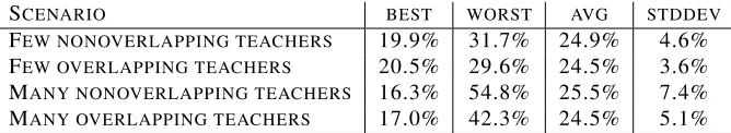
SCENARIO BEST WORST AVG STDDEV
FEW NONOVERLAPPING TEACHERS 19.9% 31.7% 24.9% 4.6% FEW OVERLAPPING TEACHERS 20.5% 29.6% 24.5% 3.6% MANY NONOVERLAPPING TEACHERS 16.3% 54.8% 25.5% 7.4% MANY OVERLAPPING TEACHERS 17.0% 42.3% 24.5% 5.1%
Table 1: Performance (test set mistake rate) of the generated teachers in the four simulated scenar-ios. Results are averaged over 10 repetitions. “best”, “worst”, and “avg” are the (average) mistake rate of the best, worst and average performing teacher, respectively. “stddev” is the standard deviation of the mistake rates, and gives an idea of the difference in performance across teachers(not across repetitions).
relevant statistics about the teachers’ performance on the test set (notice that such figures can only be computed after knowing the true labels on the test set—this information was never made available to the multiple teacher algorithm). As expected, best and worst teachers are farther apart in the nonoverlapping scenarios (correspondingly, ”stddev” figures are larger), with a larger variability in the many teacher settings. Moreover, throughout the 10 repetitions, it often happened that among the many poorly trained classifiers (as are those produced within the “many nonoverlapping” setting), a few of them turned out to be significantly accurate on the test set. Likewise, some of them happened to be even worse than random guessing.
After simulating the teachers, we implemented a simplified version of our second-version mul-tiple teacher algorithm (Algorithm 3), where the thresholdsθ2
j,t are simplified to
θ2j,t=αx⊤t A−j,1t−1xtlog(1+t), (12) andα>0 is a tunable parameter (independent ofjandt). Hence our algorithm now has two param-eters: τ∈[0,1]andα>0. The reason for this simplifiedθj,t is that the actual expression forθj,t, as it appears in Algorithm 3, is the one suggested by the theory after significant mathematical over-approximations (large deviations, H¨older’s inequality, etc.). This suggests that the exact expression forθj,t given in the pseudocode may be too conservative to work well in practice. In any event, ob-serve that the factorαlog(1+t)in (12) is a good proxy for the factor 1+4∑ti−=11Ziri+36log(Kt/δ) in the algorithm’s pseudocode, once we letαrange over the positive reals.
The following three baselines were used in our comparative study.