On Multilabel Classification and Ranking with Bandit Feedback

(1)

On Multilabel Classification and Ranking with Bandit

Feedback

Claudio Gentile [email protected]

DiSTA, Universit`a dell’Insubria via Mazzini 5

21100 Varese, Italy

Francesco Orabona [email protected]

Toyota Technological Institute at Chicago 6045 South Kenwood Avenue

60637 Chicago, IL, USA

Editor:Peter Auer

Abstract

We present a novel multilabel/ranking algorithm working in partial information settings. The algorithm is based on 2nd-order descent methods, and relies on upper-confidence bounds to trade-off exploration and exploitation. We analyze this algorithm in a partial adversarial setting, where covariates can be adversarial, but multilabel probabilities are ruled by (generalized) linear models. We showO(T1/2_log_T_{) regret bounds, which improve}

in several ways on the existing results. We test the effectiveness of our upper-confidence scheme by contrasting against full-information baselines on diverse real-world multilabel data sets, often obtaining comparable performance.

Keywords: contextual bandits, structured prediction, ranking, online learning, regret bounds, generalized linear

1. Introduction

Consider a book recommendation system. Given a customer’s profile, the system recom-mends a few possible books to the user by means of, e.g., a limited number of banners placed at different positions on a webpage. The system’s goal is to select books that the user likes and possibly purchases. Typical feedback in such systems is the actual action of the user or, in particular, what books he has bought/preferred, if any. The system cannot observe what would have been the user’s actions had other books got recommended, or had the same book ads been placed in a different order within the webpage.

Such problems are collectively referred to as learning with partial feedback. As opposed to the full information case, where the system (the learning algorithm) knows the outcome of each possible response (e.g., the user’s action for each and every possible book recom-mendation placed in the largest banner ad), in the partial feedback setting the system only observes the response to very limited options and, specifically, the option that was actually recommended.

(2)

are displayed on top of the page should somehow be more committing as a recommendation than smaller ones placed elsewhere. Moreover, it is often plausible to interpret the user feedback as a preference (if any)restricted to the displayed alternatives.

In this paper, we consider instantiations of this problem in the multilabel and learning-to-rank settings. Learning proceeds in rounds: in roundt, the algorithm receives an instance xt and outputs an ordered subset ˆYt of labels from a finite set of possible labels [K] = {1,2, . . . , K}. Restrictions might apply to the size of ˆYt(due, e.g., to the number of available

slots in the webpage, or to the specifics of the targeted user). The set ˆYt corresponds to the

aforementioned recommendations, and is intended to approximate the true set of preferences associated with xt. However, the latter set is never observed. In its stead, the algorithm

receivesYt∩Yˆt, whereYt⊆[K] is a noisy version of the true set of user preferences onxt.

When we are restricted to|Yˆt|= 1 for allt, this becomes a multiclass classification problem

with bandit feedback—see below.

1.1 Related Work

This paper lies at the intersection between online learning with partial feedback and mul-tilabel classification/ranking. Both fields include a substantial amount of work, so we can hardly do it justice here. In the sequel, we outline some of the main contributions in the two fields, with an emphasis on those we believe are the most related to this paper.

A well-known tool for facing the problem of partial feedback in online learning is to trade off exploration and exploitation through upper confidence bounds. This technique has been introduced by Lai and Robbins (1985), and can by now be considered a standard tool. In the so-called banditsetting with contextual information (sometimes called bandits with side information or bandits with covariates, e.g., Auer 2002; Dani et al. 2008; Filippi et al. 2010; Crammer and Gentile 2011; Krause and Ong 2011, and references therein) an online algorithm receives at each time step a context (typically, in the form of a feature vectorx) and is compelled to select an action (e.g., a label), whose goodness is quantified by a predefined loss function. Full information about the loss function (one that would perhaps allow to minimize the total loss over the contexts seen so far) is not available. The specifics of the interaction model determines which pieces of loss will be observed by the algorithm, e.g., the actual value of the loss on the chosen action, some information on more profitable directions on the action space, noisy versions thereof, etc. The overall goal is to compete against classes of functions that map contexts to (expected) losses in a regret sense, that is, to obtain sublinear cumulative regret bounds.

(3)

is considered by Langford and Zhang (2008), where a T2/3 regret bound has been proven under i.i.d. assumptions. Linear multiclass classification problems with bandit feedback are considered by, e.g., Kakade et al. (2008); Crammer and Gentile (2011); Hazan and Kale (2011), where either T2/3 orT1/2 or even logarithmic regret bounds are proven, depending on the noise model and the underlying loss functions.

All the above papers do not consider structured action spaces, where the learner is allowed to selectsetsof actions, which is more suitable to multilabel and ranking problems. Along these lines are the papers by Hazan and Kale (2009); Streeter et al. (2009); Kale et al. (2010); Slivkins et al. (2010); Shivaswamy and Joachims (2012); Amin et al. (2011). The general problem of online minimization of a submodular loss function under both full and bandit information without covariates is considered by Hazan and Kale (2009), achieving a regretT2/3 in the bandit case. Streeter et al. (2009) consider the problem of online learning of assignments, where at each round an algorithm is requested to assign positions (e.g., rankings) to sets of items (e.g., ads) with given constraints on the set of items that can be placed in each position. Their problem shares similar motivations as ours but, again, the bandit version of their algorithm does not explicitly take side information into account, and leads to aT2/3regret bound. Another paper with similar goals but a different mathematical model is by Kale et al. (2010), where the aim is to learn a suitable ordering (an “ordered slate”) of the available actions. Among other things, the authors prove aT1/2 regret bound in the bandit setting with a multiplicative weight updating scheme. Yet, no contextual information is incorporated. Slivkins et al. (2010) motivate the ability of selecting sets of actions by a problem of diverse retrieval in large document collections which are meant to live in a general metric space. In contrast to our paper, that approach does not lead to strong regret guarantees for specific (e.g., smooth) loss functions. Shivaswamy and Joachims (2012) use a simple linear model for the hidden utility function of users interacting with a web system and providing partial feedback in any form that allows the system to make significant progress in learning this function (this is called anα-informative feedback by the authors). Under these assumptions, a regret bound ofT1/2is again provided that depends on the degree of informativeness of the feedback, as measured by the progress made during the learning process. It is experimentally argued that this feedback is typically made available by a user that clicks on relevant URLs out of a list presented by a search engine. Despite the neatness of the argument, no formal effort is put into relating this information to the context information at hand or, more generally, to the way data are generated. The recent paper by Amin et al. (2011) investigates classes of graphical models for contextual bandit settings that afford richer interaction between contexts and actions leading again to aT2/3 regret bound.

(4)

setting we are interested in (or, if they do, we do not see it in the current version of their paper). Moreover, being very general in scope, that paper is missing a tight dependence of the regret bound on the number of available actions, which can be very large in structured action spaces. Progress in this directions has very recently been made by Bart´ok (2013), where the dependence on the number of actions is replaced by a quantity depending on the structure of the action space in the locally observable game. Yet, no side information is considered in that paper. The paper by Agarwal (2013) investigates multiclass selective sampling settings (similar to Cavallanti et al., 2011; Cesa-Bianchi et al., 2009; Dekel et al., 2012; Orabona and Cesa-Bianchi, 2011) with essentially the same generalized linear models as the ones we consider here. As such, that paper is close to ours only from a technical viewpoint.

The literature on multilabel learning and learning to rank is overwhelming. The wide at-tention this literature attracts is often motivated by its web-search-engine or recommender-system applications, and many of the papers are experimental in nature. Relevant references include the work by Tsoumakas et al. (2011); Furnkranz et al. (2008); Dembczynski et al. (2012), along with references therein. Moreover, when dealing with multilabel, the typical assumption is full supervision, an important concern being modeling correlations among classes. In contrast to that, the specific setting we are considering here need not face such a modeling issue (Dembczynski et al., 2012). The more recent work by Wang et al. (2012) reduces any online algorithm working on pairwise loss functions (like a ranking loss) to a batch algorithm with generalization bound guarantees. But, again, only fully supervised settings are considered. Other related references are the papers by Herbrich et al. (2000); Freund et al. (2003), where learning is by pairs of examples. Yet, these approaches need i.i.d. assumptions on the data, and typically deliver batch learning procedures. Finally, more re-cent efforts related to proving consistency of pairwise ranking methods are Cl´emen¸con et al. (2005); Cossock and Zhang (2006); Duchi et al. (2010); Buffoni et al. (2011); Lan et al. (2012) where, unlike this paper, multi-level user ratings are assumed to be available.

To summarize, whereas we are technically closer to the linear modeling approaches by Auer (2002); Dani et al. (2008); Dekel et al. (2012); Crammer and Gentile (2011); Filippi et al. (2010); Abbasi-Yadkori et al. (2011); Krause and Ong (2011); Bart´ok and Szepesv´ari (2012); Agarwal (2013), from a motivational standpoint we are perhaps closest to Streeter et al. (2009); Kale et al. (2010); Shivaswamy and Joachims (2012).

1.2 Our Results

(5)

2009; Abbasi-Yadkori et al. 2011; Krause and Ong 2011), we are not assuming the algorithm is observing a noisy version of the risk function on the currently selected action. In fact, when a generalized linear model is adopted, the mapping context-to-risk turns out to be nonconvex in the parameter space. Furthermore, when operating on structured action spaces this more traditional form of bandit model does not seem appropriate to capture the typical user preference feedback. Our approach is based on having the loss decoupled from the label generating model, the user feedback being a noisy version of the gradient of

a surrogate convex loss associated with the model itself. As a consequence, the algorithm

is not directly dealing with the original loss when making exploration. In this sense, we are more similar to the multiclass bandit algorithm by Crammer and Gentile (2011). Yet, our work is a substantial departure from Crammer and Gentile’s (2011) in that we lift their machinery to nontrivial structured action spaces, and we do so by means of generalized linear models. On one hand, these extensions pose several extra technical challenges; on the other, they provide additional modeling power and practical advantage.

Though the emphasis is on theoretical results, we also validate our algorithms on real-world multilabel data sets under several experimental conditions: data set size, label set size, loss functions, training mode and performance (online vs. batch), label generation model (linear vs. logistic). Under all such conditions, our algorithms are contrasted against the corresponding multilabel/ranking baselines that operate with full information, often showing (surprisingly enough) comparable prediction performance.

1.3 Structure of the Paper

The paper is organized as follows. In Section 2 we introduce our learning model, our first loss function, the label generation model, and some preliminary results and notation used throughout the rest of the paper. In Section 3 we describe our partial feedback algorithm working under the loss function introduced in Section 2, along with the associated regret analysis. In Section 4 we show that a very similar machinery applies to ranking with partial feedback, where the loss function is a kind of pairwise ranking loss (with partial feedback). Similar regret bounds are then presented that work under additional modeling restrictions. In Section 5 we provide our experimental comparison. Section 6 gives proof ideas and technical details. The paper is concluded with Section 7, where possible directions for future research are mentioned.

2. Model and Preliminaries

We consider a setting where the algorithm receives at time t the side information vector xt ∈ Rd, is allowed to output a (possibly ordered) subset1 Yˆt ⊆ [K] of the set of possible

labels, then the subset of labelsYt⊆[K] associated withxtis generated, and the algorithm

gets as feedback ˆYt∩Yt. The loss suffered by the algorithm may take into account several

things: thedistancebetweenYtand ˆYt(both viewed as sets), as well as thecost for playing

ˆ

Yt. The cost c( ˆYt) associated with ˆYt might be given by the sum of costs suffered on

each class i∈ Yˆt, where we possibly take into account the order in which i occurs within

ˆ

Yt (viewed as an ordered list of labels). Specifically, given constant a ∈ [0,1] and costs

(6)

c = {c(i, s), i = 1, . . . , s, s ∈ [K]}, such that 1 ≥ c(1, s) ≥ c(2, s) ≥ . . . c(s, s) ≥ 0, for all s∈[K], we consider the loss function

`a,c(Yt,Yˆt) =a|Yt\Yˆt|+ (1−a) X

i∈_Ytˆ\Yt

c(ji,|Yˆt|),

where ji is the position of class i in ˆYt, and c(ji,·) depends on ˆYt only through its size |Yˆt|. In the above, the first term accounts for the false negative mistakes, hence there is no

specific ordering of labels therein. The second term collects the loss contribution provided by all false positive classes, taking into account through the costs c(ji,|Yˆt|) the order in

which labels occur in ˆYt. The constant a serves as weighting the relative importance of

false positive vs. false negative mistakes.2 As a specific example, suppose that K = 10, the costs c(i, s) are given by c(i, s) = (s−i+ 1)/s, i = 1, . . . , s, the algorithm plays the ordered list ˆYt = (4,3,6), but Yt is the (unordered) set {1,3,8}. In this case,|Yt\Yˆt|= 2,

and P

i∈_Ytˆ\Ytc(ji,|Yˆt|) = 3/3 + 1/3, i.e., the cost for mistakenly playing class 4 in the top

slot of ˆYt is more damaging than mistakenly playing class 6 in the third slot. In the special

case when all costs are unitary, there is no longer need to view ˆYtas an ordered collection,

and the above loss reduces to a standard Hamming-like loss between sets Yt and ˆYt, i.e.,

a|Yt\Yˆt|+ (1−a)|Yˆt\Yt|. Notice that the partial feedback ˆYt∩Yt allows the algorithm

to know which of the chosen classes in ˆYt are good or bad (and to what extent, because of

the selected ordering within ˆYt).

The reader should also observe the asymmetry between the label set ˆYtproduced by the

algorithm and the true label setYt: the algorithm predicts an ordered set of labels, but the

true set of labels is unordered. In fact, it is often the case in, e.g., recommender system practice, that the user feedback does not contain preference information in the form of an ordered set of items. Still, in such systems we would like to get back to the user with an appropriate ranking over the items.

Working with the above loss function makes the algorithm’s output ˆYt become a ranked

list of classes, where ranking isrestrictedto the deemed relevant classes only. In this sense, the above problem can be seen as a partial information version of the multilabel ranking problem (see the work by Furnkranz et al., 2008, and references therein). In a standard multilabel ranking problem a classifier has to provide for any given instance xt, both a

separation between relevant and irrelevant classes and a ranking of the classes within the two sets (or, perhaps, over the whole set of classes, as long as ranking is consistent with the relevance separation). In our setting, instead, ranking applies to the selected classes only, but the information gathered by the algorithm while training is partial. That is, only a relevance feedback among the selected classes is observed (the setYt∩Yˆt), but no supervised

ranking information (e.g., in the form of pairwise preferences) is provided to the algorithm within this set. Alternatively, we can think of a ranking framework where restrictions on the size of ˆYtare set by an exogenous (and possibly time-varying) parameter of the problem,

and the algorithm is required to provide a ranking complying with these restrictions. In this sense, an alternative interpretation of the ranking-sensitive term P

i∈Ytˆ\Ytc(ji,|Yˆt|) in

`a,c(Yt,Yˆt) is a Discounted Cumulative Gain (DCG) difference between the optimal ranking

(7)

(i.e., the one sorting the |Yt| classes in Yt according to decreasing value of c(i,|Yˆt|)) and

the actual ranking contained in ˆYt, the discounting function being just the coefficients

c(i,|Yˆt|), i = 1, . . .|Yˆt|. DCG is a standard metric for measuring the effectiveness of Web

search engine algorithms (e.g., Jarvelin and Kekalainen, 2002).

Another important concern we would like to address with our loss function `a,c is to

avoid combinatorial explosions due to the exponential number of possible choices for ˆYt.

As we shall see below, this is guaranteed by the chosen structure for costs c(i, s). Another loss function providing similar guarantees (though with additional modeling restrictions) is the (pairwise) ranking loss considered in Section 4, where more on the connection to the ranking setting with partial feedback is given.

The problem arises as to which noise model we should adopt so as to encompass sig-nificant real-world settings while at the same time affording efficient implementation of the resulting algorithms. For any subset Yt ⊆ [K], we let (y1,t, . . . , yK,t) ∈ {0,1}K be the

corresponding indicator vector. Then it is easy to see that

`a,c(Yt,Yˆt) =a X

i /∈_Ytˆ

yi,t+ (1−a) X

i∈_Ytˆ

c(ji,|Yˆt|) (1−yi,t)

=a

K X

i=1

yi,t+ (1−a) X

i∈_Ytˆ

c(ji,|Yˆt|)−

a

1−a +c(ji,|Yˆt|)

yi,t

.

Moreover, because the first sum does not depend on ˆYt, for the sake of optimizing over ˆYt

(but also for the sake of defining the regretRT—see below) we can equivalently define

`a,c(Yt,Yˆt) = (1−a) X

i∈_Ytˆ

c(ji,|Yˆt|)−

a

1−a+c(ji,|Yˆt|)

yi,t

. (1)

Note that the algorithm can evaluate the value of this loss, using the feedback received. LetPt(·) be a shorthand for the conditional probabilityP(· |xt), where the side information

vectorxt can in principle be generated by an adaptive adversary as a function of the past.

Then

Pt(y1,t, . . . , yK,t) =P(y1,t, . . . , yK,t|xt).

We will assume that the marginals Pt(yi,t= 1) satisfy3

Pt(yi,t= 1) =

g(−u>_i xt)

g(u>_i xt) +g(−u>i xt)

, i= 1, . . . , K, (2)

for some K vectors u1, . . . ,uK ∈ Rd, and a (known) function g : D ⊆ R → R+, that

is the negative derivative of a suitable convex and nonincreasing function. The model is well defined if u>_i x∈ D for all iand all x∈ Rd _{chosen by the adversary. We assume for}

the sake of simplicity that ||xt|| = 1 for all t. Notice that here the variables yi,t need not

be conditionally independent. We are only defining a family of allowed joint distributions

3. The reader familiar with generalized linear models will recognize the derivative of the functionp(∆) =

g(−∆)

g(∆)+g(−∆) as the (inverse) link function of the associated canonical exponential family of distributions

(8)

Pt(y1,t, . . . , yK,t) through the properties of their marginalsPt(yi,t). A classical result in the

theory of copulas (Sklar, 1959) makes one derive all allowed joint distributions starting from the corresponding one-dimensional marginals. It is also important to point out the arbitrary dependence of xt on the past, since the typical scenarios we are modeling here (human

interaction) are producing data sequences which are nonstationary in nature, implying that traditional statistical inference methods (e.g., empirical risk minimization) should be used cautiously.

Our algorithm will be based on the loss function L, which is such that the function g above is equal to the negative derivative of L. For instance, if L is the square loss L(∆) = (1−∆)2_/_{2, then}_g_{(∆) = 1}₋_{∆, resulting in}

Pt(yi,t= 1) = (1 +u>i xt)/2, under the

assumption D = [−1,1]. If L is the logistic loss L(∆) = ln(1 +e−∆), then g(∆) = _e∆1₊₁,

and Pt(yi,t = 1) = eu >

ixt/(eu>ixt + 1), with domain D = R. Observe that in both cases Pt(yi,t= 1) is an increasing function of u>i xt. This will be true in general.

Set for brevity ∆i,t =u>i xt. Taking into account (1), this model allows us to write the

(conditional) expected loss of the algorithm playing ˆYt as

Et[`a,c(Yt,Yˆt)] = (1−a) X

i∈_Ytˆ

c(ji,|Yˆt|)−

a

1−a+c(ji,|Yˆt|)

pi,t

, (3)

where we introduced the shorthands

pi,t =p(∆i,t), p(∆) =

g(−∆) g(∆) +g(−∆),

and the expectation Etin (3) is w.r.t. the generation of labels Yt, conditioned on bothxt,

and all previous xand Y.

A key aspect of this formalization is that the Bayes optimal ordered subset

Y_t∗ = argmin_Y₌₍_j1,j2_,...,j

|Y|)⊆[K]Et[`a,c(Yt, Y)]

can be computed efficiently when knowing ∆1,t, . . . ,∆K,t. This is handled by the next

lemma. In words, this lemma says that, in order to minimize (3), it suffices to try out all possible sizes s= 0,1, . . . , K forY_t∗ and, for each such value, determine the sequence Y_s,t∗ that minimizes (3) over all sequences of sizes. In turn,Y_s,t∗ can be computed just by sorting classesi∈[K] in decreasing order ofpi,t, sequence Ys,t∗ being given by the first sclasses in

this sorted list.

Lemma 1 With the notation introduced so far, let pi1,t ≥pi2,t ≥ . . . piK,t be the sequence

of pi,t sorted in nonincreasing order. Then we have that

Y_t∗= argmin_s₌₀_,₁_,...KEt[`a,c(Yt, Ys,t∗)],

where Y_s,t∗ = (i1, i2, . . . , is), and Y0∗,t=∅.

Proof First observe that, for any given size s, the sequence Y_s,t∗ must contain the s top-ranked classes in the sorted order of pi,t. This is because, for any candidate sequence Ys= {j1, j2, . . . , js}, we haveEt[`a,c(Yt∗, Ys)] = (1−a) Pi∈Ys

c(ji, s)−

a

1−a+c(ji, s)

pi,t

(9)

there existsi∈Ys which is not among thes-top ranked ones, then we could replace classi

in positionji within Ys with class k /∈Ys such that pk,t> pi,t obtaining a smaller loss.

Next, we show that the optimal ordering withinY_s,t∗ is precisely ruled by the nonincreas-ing order ofpi,t. By the sake of contradiction, assume there are iand kin Ys,t∗ such thati

precedes kinY_s,t∗ butpk,t> pi,t. Specifically, letibe in position j1 and kbe in position j2 withj1 < j2and such thatc(j1, s)> c(j2, s). Then, disregarding the common (1−a)-factor, switching the two classes withinY_s,t∗ yields an expected loss difference of

c(j1, s)−

a

1−a +c(j1, s)

pi,t+c(j2, s)−

a

1−a+c(j2, s)

pk,t −c(j1, s)−

a

1−a+c(j1, s)

pk,t

−c(j2, s)−

a

1−a +c(j2, s)

pi,t

= (pk,t−pi,t) (c(j1, s)−c(j2, s))>0,

sincepk,t> pi,t andc(j1, s)> c(j2, s). Hence switching would get a smaller loss which leads as a consequence toY_s,t∗ = (i1, i2, . . . , is).

Notice the way costs c(i, s) influence the Bayes optimal computation. We see from (3) that placing class iwithin ˆYtin positionji is beneficial (i.e., it leads to a reduction of loss)

if and only if pi,t > c(ji,|Yˆt|)/(1−aa +c(ji,|Yˆt|)). Hence, the higher is the slot ij in ˆYt the

larger should be pi,t in order for this inclusion to be convenient.4

It is Y_t∗ above that we interpret as the true set of user preferences onxt. We would like

to compete againstY_t∗ in a cumulative regret sense, i.e., we would like to bound

RT = T X

t=1

Et[`a,c(Yt,Yˆt)]−Et[`a,c(Yt, Yt∗)]

with high probability.

We use a similar but largely more general analysis than Crammer and Gentile (2011)’s to devise an online second-order descent algorithm whose updating rule makes the comparison vector U = (u1, . . . ,uK) ∈ RdK defined through (2) be Bayes optimal w.r.t. a surrogate

convex lossL(·) such thatg(∆) =−L0(∆). Observe that the expected loss function defined in (3) is, generally speaking, nonconvex in the margins ∆i,t (consider, for instance the

logistic caseg(∆) = _e∆1₊₁). Thus, we cannot directly minimize this expected loss.

3. Algorithm and Regret Bounds

In Figure 2 is our bandit algorithm for (ordered) multiple labels. In order to acquaint the reader with this algorithm, a simplified version of it is first presented (Figure 1) which applies to the linear model p(∆) = 1+∆₂ ,g(∆) = 1−∆, under the simplifying assumption

||ui|| ≤1, fori∈[K].

4. Notice that this depends on the actual size of ˆYt, so we cannot decompose this problem intoK

inde-pendent problems. The decomposition does occur if the costsc(i, s) are constants, independent ofiand

(10)

Parameters:

• Loss parametersa∈[0,1], and cost valuesc(i, s);

• Confidence levelδ∈[0,1].

Initialization: Ai,0=I∈ Rd×d,i= 1, . . . , K, wi,1= 0∈ Rd, i= 1, . . . , K;

Fort= 1,2. . . , T :

1. Get instancext∈ Rd : ||xt||= 1; 2. Fori∈[K], set∆b_i,t0 =x>_tw0_i,t, where

w0i,t=



    

    

wi,t ifw>i,txt∈[−1,1],

wi,t−

w>_i,txt−1

x>

tA

−1 i,t−1xt

A−_i,t1₋₁xt ifw>i,txt>1,

wi,t−

w>

i,txt+1 x>

tA

−1 i,t−1xt

A−_i,t1₋₁xt ifw>i,txt<−1;

3. Output

ˆ

Yt= argmin Y=(j1,j2,...j|Y|)⊆[K]

X

i∈Y

c(ji,|Y|)− a

1−a +c(ji,|Y|)

b

pi,t

!

,

where

b

pi,t =1 + [∆b

0

i,t+i,t][−1,1]

2 ,

2i,t =x>tA−

1

i,t−1xt

1 + 4dln

1 +t−1 d

+ 48 lnK(t+ 4) δ

;

4. Get feedbackYt∩Yˆt; 5. Fori∈[K], update:

Ai,t=Ai,t−1+|si,t|xtx>t, wi,t+1=w0i,t−A

−1

i,t∇i,t, where

si,t=



 

 

1 ifi∈Yt∩Ytˆ,

−1 ifi∈_Yˆ_t_\_Y_t_{= ˆ}_Y_t_\₍_Y_t_∩_Yˆ_t_), 0 otherwise;

and

∇i,t= (si,t∆b0_i,t−1)si,txt.

Figure 1: The partial feedback algorithm in the (ordered) multiple label setting—the linear model case.

Both algorithms are based on replacing the unknown model vectors u1, . . . ,uK with

(11)

sim-Parameters:

• Loss parametersa∈[0,1], and cost valuesc(i, s);

• IntervalD= [−R, R], functiong : D→ R;

• Confidence levelδ∈[0,1], and norm upper boundU >0.

Initialization: Ai,0=I∈ Rd×d,i= 1, . . . , K, wi,1= 0∈ Rd, i= 1, . . . , K;

Fort= 1,2. . . , T :

1. Get instancext∈ Rd : ||xt||= 1; 2. Fori∈[K], set∆b_i,t0 =x>_tw0_i,t, where

w0_i,t=

          

wi,t ifw>i,txt∈[−R, R],

wi,t−

w>_i,txt−R x>

tA

−1 i,t−1xt

A−_i,t1₋₁xt ifw>i,txt> R,

wi,t−

w>_i,txt+R

x>

tA

−1 i,t−1xt

A−_i,t1₋₁xt ifw>i,txt<−R;

3. Output

ˆ

X

i∈Y

c(ji,|Y|)−

a

1−a +c(ji,|Y|)

b pi,t ! , where b

pi,t =p

[∆b0_i,t+i,t]D

=

g−[∆b0_i,t+i,t]D

g[∆b0_i,t+i,t]D

+g−[∆b0_i,t+i,t]D

,

2_i,t =x>_tA−_i,t1₋₁xt

U2+ d c

0

L (c00

L)2 ln

1 + t−1 d +12 c00 L _c0 L c00 L

+ 3L(−R)

lnK(t+ 4) δ

;

4. Get feedbackYt∩Yˆt; 5. Fori∈[K], update:

Ai,t=Ai,t−1+|si,t|xtx>t, wi,t+1=w0i,t− 1 c00

L

A−_i,t1∇i,t,

where

si,t=



 

 

1 ifi∈Yt∩Yˆt,

−1 ifi∈Ytˆ \Yt= ˆYt\(Yt∩Ytˆ), 0 otherwise;

and

∇i,t=∇wL(si,tw>xt)|w=w0

i,t =−g(si,t∆b 0

i,t)si,txt.

(12)

ilar constraints we set for theui vectors. For the sake of brevity, we let∆b0_i,t =x>_t w0_i,t, and

∆i,t=u>i xt,i∈[K].

The algorithms use ∆b0_i,t as proxies for the underlying ∆_i,t according to the (upper

confidence) approximation scheme ∆i,t ≈[∆b0_i,t +_i,t]_D, where _i,t ≥0 is a suitable

upper-confidence level for class i at time t, and [·]D denotes the clipping-to-D operation: if D=

[−R, R], then

[x]D = 

 

 

R ifx > R x if−R≤x≤R

−R ifx <−R.

The algorithms’ prediction at time t has the same form as the computation of the Bayes optimal sequence Y_t∗, where we replace the true (and unknown) pi,t = p(∆i,t) with the

corresponding upper confidence proxy

b

pi,t =p([∆b0_i,t+_i,t]_D),

being

ˆ

X

i∈Y

c(ji,|Y|)−

a

1−a+c(ji,|Y|)

b

pi,t

!

.

Computing ˆYt above can be done by mimicking the computation of the Bayes optimal

ordered subsetY_t∗(just replacepi,tbybpi,t). From a computational viewpoint, this essentially

amounts to sorting classes i∈[K] in decreasing value ofpbi,t, i.e., order ofKlogK running

time per prediction. Thus the algorithms are producing a ranked list of relevant classes based on upper-confidence-corrected scoresp_bi,t. Classiis deemed relevant and ranked high

among the relevant ones when either ∆b0_i,t is a good approximation to ∆_i,t and p_i,t is large,

or when the algorithms are not very confident on their own approximation abouti(that is, the upper confidence leveli,t is large).

Specifically, the algorithm in Figure 1 receives in input the loss parametersaandc(i, s), and the desired confidence levelδ, and maintains both K positive definite matrices Ai,t of

dimension d (initially set to the d×d identity matrix), and K weight vectors wi,t ∈ Rd

(initially set to the zero vector). At each time step t, upon receiving the d-dimensional instance vector xt the algorithm uses the weight vectors wi,t to compute the prediction

vectors w0_i,t. These vectors can easily be seen as the result of projectingwi,t onto interval

[−1,1] w.r.t. the distance functiondi,t−1, i.e.,

w0_i,t = argmin

w∈Rd_:_w>_xt_∈[−1_,_1]

di,t−1(w,wi,t), i∈[K],

where

di,t−1(u,w) = (u−w)>Ai,t−1(u−w).

Vectorsw0_i,tare then used to produce prediction values∆b0_i,tinvolved in the upper-confidence

calculation of the predicted ordered subset ˆYt⊆[K]. Next, the feedbackYt∩Yˆtis observed,

(13)

classesi∈Yˆt\Yt (signsi,t =−1), and leaves all remaining classesi /∈Yˆt unchanged (sign

si,t = 0). Promotion of classion xtimplies that if the new vector xt+1 is close to xt then

iwill be ranked higher onxt+1. The updatewi,t0 →wi,t+1 is based on the gradients ∇i,t of

the square loss function L(∆) = (1−∆)2/2. On the other hand, the update Ai,t−1 → Ai,t

uses the rank-one matrix5_x

tx>t. The matrixAi,t−1is used to calculate the upper confidence level on each prediction. Matrix Ai,t−1 is the empirical covariance matrix of the samples on which we received some feedback, either positive (si,t = 1) or negative (si,t =−1), and

is used in the expression for the confidence 2_i,t involving the quadratic form x>_t A−1_i,t₋₁xt.

Notice that 2_i,t will be small when the current sample xt is in the span of the previous

samples on which we received feedback, and will be large otherwise. In both the update of w0_i,t and the one involvingAi,t−1, the reader should observe the role played by the signssi,t.

The algorithm contained in Figure 2 is just a more general version of the one in Figure 1, where we also receive in input the specifics of the generalized linear model through the model function g(·) and the associated margin domain D= [−R, R], and the norm upper bound U, such that kuik ≤ U for all i ∈ [K]. The update w0_i,t → wi,t+1 in Figure 2 is based on the gradients ∇_i,t of a loss functionL(·) satisfying L0(∆) =−g(∆). On the other hand, the update Ai,t−1 → Ai,t uses again the rank-one matrix xtx>t. The constants c0L

and c00_L occurring in the expression for 2_i,t in Figure 2 are related to smoothness properties of L(·). In particular, 2_i,t in Figure 1 is obtained from 2_i,t in Figure 2 by setting R = 1, L(−R) =L(−1) = 0, along with c0_L= 4 andc00_L= 1, as explained in the next theorem.6

Theorem 2 Let L : D = [−R, R] ⊆ R → R+ _{be a} _C2₍_D₎ _{convex and nonincreasing}

function of its argument,(u1, . . . ,uK)∈ RdK be defined in (2) with g(∆) =−L0(∆) for all

∆∈D, and such thatkuik ≤U for alli∈[K]. Assume there are positive constants cL, c0_L

and c00_L such that

i. L0(∆)L₍_L000(−∆)+_(∆)+_LL0_(−∆))00(∆)L20(−∆) ≥ −cL,

ii. (L0(∆))2 ≤c0_L, iii. L00(∆)≥c00_L

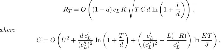
simultaneously hold for all ∆ ∈ D. Then the cumulative regret RT of the algorithm in

Figure 2 satisfies, with probability at least1−δ,

RT =O (1−a)cLK s

T C dln

1 +T d

!

,

where

C=O

U2+ d c 0

L

(c00_L)2 ln

1 +T d

+

c0_L (c00_L)2 +

L(−R) c00_L

lnKT δ

.

5. The rank-one update is based onxtx>t rather than∇i,t∇

>

i,t, as in , e.g., the paper by Hazan et al. (2007). This is due to technical reasons that will be made clear in Section 6. This feature tells this algorithm slightly apart from the Online Newton step algorithm (Hazan et al., 2007), which is the starting point of our analysis. The very same comment applies to the algorithm in Figure 2.

(14)

It is easy to see that when L(·) is the square loss L(∆) = (1−∆)2/2 and D= [−1,1], we have cL = 1/2, c0_L= 4 and c00_L = 1; when L(·) is the logistic lossL(∆) = ln(1 +e−∆) and

D= [−R, R], we have cL= 1/4, c0L≤1 andc00L= 2(1+cosh(1 R)), where cosh(x) =

ex₊_e−x

2 . The following remarks are in order at this point.

Remark 3 A drawback of Theorem 2 is that, in order to properly set the upper confidence levelsi,t, we assume prior knowledge of the norm upper bound U. Because this information

is often unavailable, we present here a simple modification to the algorithm that copes with this limitation, similar to the one proposed in Orabona and Cesa-Bianchi (2011). We change the definition of 2_i,t in Figure 2 to

2_i,t= max

(

x>A−1_i,t₋₁x

2d c0_L (c00_L)2 ln

1 +t−1 d

+12 c00_L

c0_L

c00_L + 3L(−R)

lnK(t+ 4) δ

,4R2

)

,

that is, we substitute U2 by d c

0 L

(c00_L)2 ln 1 + t−1_d

, and cap the maximal value of 2_i,t to 4R2. This immediately leads to the following result.7

Theorem 4 With the same assumptions and notation as in Theorem 2, if we replace 2_i,t

as explained above we have that, with probability at least 1−δ, RT satisfies

RT =O (1−a)cLK s

T C dln

1 +T d

+ (1−a)cLK R d

exp

(c00_L)2U2 c0_Ld

−1

!

.

Remark 5 From a computational standpoint, the most demanding operation in Figure 2

is computing the upper confidence levels i,t involving the inverse matrices A−1i,t−1, i∈[K].

Note that the matrices can be safely inverted because they are full rank, being initialized

with identity matrices. The matrix inversion can be done incrementally in O(K d2) time

per round. This can be hardly practical if both dandK are large. In practice (as explained, e.g., by Crammer and Gentile, 2011), one can use an approximated version of the algorithm

which maintains diagonal matrices Ai,t instead of full ones. All the steps remain the same

except Step 5 of Algorithm 2 where one defines the rth diagonal element of matrix Ai,t as

(Ai,t)r,r= (Ai,t−1)r,r+x2r,t, beingxt= (x1,t, x2,t, . . . , xr,t, . . . , xK,t)>. The resulting running

time per round (including prediction and update) becomes O(dK+KlogK). In fact, when

a limitation on the size of Yˆt is given, the running time may be further reduced, see Remark

8.

4. On Ranking with Partial Feedback

As Lemma 1 points out, when the cost values c(i, s) in the loss function `a,c are strictly

decreasing i.e., c(1, s) > c(2, s) > . . . > c(s, s), for all s ∈ [K], then the Bayes optimal ordered sequenceY_t∗ onxtis unique can be obtained by sorting classes in decreasing values

ofpi,t, and then decide on a cutoff point8induced by the loss parameters, so as to tell relevant

classes apart from irrelevant ones. In turn, because p(∆) = _g_(∆)+g(−∆)_g_(−∆) is increasing in ∆,

7. The proof is deferred to Section 6.

(15)

this ordering corresponds to sorting classes in decreasing values of ∆i,t. Now, if parameter

a in `a,c is very close9 to 1, then |Yt∗|=K, and the algorithm itself will produce ordered

subsets ˆYt such that |Yˆt| = K. Moreover, it does so by receiving full feedback on the

relevant classes at time t (since Yt∩Yˆt = Yt). As is customary (e.g., Dembczynski et al.

2012), one can view any multilabel assignment Y = (y1, . . . , yK) ∈ {0,1}K as a ranking

among the K classes in the most natural way: i precedes j if and only if yi > yj. The

(unnormalized) ranking loss function `rank(Y, f) between the multilabel Y and a ranking

functionf : Rd_{→ R}K_{, representing degrees of class relevance sorted in a decreasing order}

fj1(xt)≥fj2(xt)≥. . .≥fjK(xt)≥0, counts the number of class pairs that disagree in the

two rankings:

`rank(Y, f) =

X

i,j∈[K] :yi>yj

{fi(xt)< fj(xt)}+1₂{fi(xt) =fj(xt)}

,

where {. . .} is the indicator function of the predicate at argument. As pointed out by Dembczynski et al. (2012), the ranking functionf(xt) = (p1,t, . . . , pK,t) is also Bayes optimal

w.r.t. `rank(Y, f),no matter ifthe class labelsyiare conditionally independent or not. Hence

we can use the algorithm in Figure 2 withaclose to 1 for tackling ranking problems derived from multilabel ones, when the measure of choice is`rank and the feedback is full.

We now consider a partial information version of the above ranking problem. Suppose that at each timet, the environment discloses bothxtand a maximalsizeStfor the ordered

subset ˆYt = (j1, j2, . . . , j|_Ytˆ|) (both xt and St can be chosen adaptively by an adversary).

Here St might be the number of available slots in a webpage or the maximal number of

URLs returned by a search engine in response to queryxt. Then it is plausible to compete

in a regret sense against the best time-toffline ranking of the form f∗(xt) =f∗(xt;St) = (f1∗(xt), f2∗(xt), . . . , fK∗(xt)),

where the number of strictly positivef_i∗(xt) values is at mostSt. Further, the ranking loss

could be reasonably restricted to count the number of class pairs disagreeing within ˆYtplus

a quantity related to the number of false negative mistakes. If ˆYt is the sequence of length

St associated with a ranking function f, we consider the loss function `p−rank,t (“partial

information `rank at timet”)

`p−rank,t(Y, f) =

X

i,j∈_Ytˆ _:_yi>yj

+St|Yt\Yˆt|.

In this loss function, the factorStmultiplying|Yt\Yˆt|serves as balancing the contribution of

the double sumP

i,j∈_Ytˆ _:_yi>yj (potentially involving a quadratic number of terms) with the

contribution of false negative mistakes|Yt\Yˆt|. As for loss`a,c, we can rewrite`p−rank,t(Y, f)

as

`p−rank,t(Y, f) =

X

i,j∈Ytˆ :yi>yj

−St|Yt∩Yˆt|+St|Yt|,

9. Ifa= 1, the algorithm only cares about false negative mistakes, the best strategy being always predicting

ˆ

(16)

where the first two terms can be calculated by the algorithm, and the last one does not depend on ˆYt. For convenience, we will interchangeably use the notations`p−rank,t(Y, f) and

`p−rank,t(Y,Yˆt), whenever it is clear from the surrounding context that ˆYt is the sequence

corresponding tof.

The next lemma10 is the ranking counterpart to Lemma 1. It shows that the Bayes optimal ranking for `p−rank,t is given by

f∗(xt;St) = (p01,t, p

0

2,t, . . . , p

0

K,t),

where p0_j,t = pj,t if pj,t is among the St largest values in the sequence (p1,t, . . . , pK,t), and

0 otherwise. That is, f∗(xt;St) is the function that ranks classes according to decreasing

values ofpi,t and cuts off exactly at positionSt. This is in contrast to what happens for loss

`a,c, where, depending on the cost parameters c(i, s), the cut off point can even be smaller

than the total number of available slots—see Lemma 1 and surrounding comments. In order for this result to go through, we need to restrict model (2) to the case of conditionally independent classes, i.e., to the case when

Pt(y1,t, . . . , yK,t) = Y

i∈[K]

pi,t. (4)

This is a significant departure from the full information setting, where the Bayes optimal ranking only depends on the marginal distribution values pi,t (Dembczynski et al., 2012).

Due to the interaction between the two terms in the definition of`p−rank,t, the Bayes optimal

ranking for`p−rank,tturns out to depend on both marginal and pairwise correlation values of

the joint class distribution. Assumption (4) may be avoided by maintaining O(K2) upper confidence values i,j, one for each pair (i, j), i < j, leading to an extra computational

burden which can become prohibitive even in the presence of a moderate number of classes K.

Lemma 6 With the notation introduced so far, let the joint distribution Pt(y1,t, . . . , yK,t)

factorize as in (4). Then f∗(xt;St) introduced above satisfies

f∗(xt;St) = argmin Y=(i1,i2,...ih),h≤St

Et[`p−rank,t(Yt, Y)].

If we add to the argmin of our algorithm (Step 3 in Figure 2) the further constraint|Y| ≤St

(notice that the resulting computation is still about sorting classes according to decreasing values of p_bi,t), we are defining a partial information ranking algorithm that ranks classes

according to decreasing values ofp_bi,t up to positionSt(i.e., |Yˆt|=St). Letfb(x_t, S_t) be the

resulting ranking. We can then define the cumulative regret RT w.r.t. `p−rank,t as

RT = T X

t=1

Et[`p−rank,t(Yt,fb(x_t, S_t))]−E_t[`_p₋_rank,t(Y_t, f∗(x_t, S_t)], (5)

that is, the extent to which the conditional`p−rank,t-risk offb(x_t, S_t) exceeds the one of the

Bayes optimal rankingf∗(xt;St), accumulated over time.

We have the following ranking counterpart to Theorem 2.

(17)

Theorem 7 With the same assumptions and notation as in Theorem 2, combined with the independence assumption (4), let the cumulative regret RT w.r.t. `p−rank,t be defined as in

(5). Then, with probability at least 1−δ, we have that the algorithm in Figure 2 working

witha→1and strictly decreasing cost values c(i, s)(i.e., the algorithm computing in round

t the ranking function fb(x_t, S_t)) achieves

RT =O cL s

S K T C d ln

1 +T d

!

,

where S = maxt=1,...,T St.

The proof (see Section 6) is very similar to the one of Theorem 2. This suggests that, to some extent, we are decoupling the label generating model from the loss function ` under consideration.

Remark 8 As is typical in many multilabel classification settings, the number of classesK

can be very large and/or have an inner structure (e.g., a hierarchical or DAG-like structure). It is often the case that in such a large label space, many classes are relatively rare. This has lead researchers to consider methods that are specifically tailored to leverage the label sparsity of the chosen classifier (e.g., Hsu et al. 2009 and references therein) and/or the specific structure of the set of labels (e.g., Cesa-Bianchi et al. 2006a; Bi and Kwok 2011, and references therein). Though our algorithm is not designed to exploit the label structure, we would like to stress that the restriction |Yˆt| ≤St≤S in Theorem 7 allows us to replace

the linear dependence on the total number of classes K (which is often much larger thanS)

by √SK. It is very easy to see that this restriction would bring similar benefits to Theorem 2.

In fact, the above restriction is not only beneficial from a “statistical” point of view, but also from a computational one. As is by now standard, algorithms like the one in Figure 2 can easily be cast in dual variables (i.e., in a RKHS). This comes with at least two consequences:

1. We can depart from the (generalized) linear modeling assumption (2), and allow for more general nonlinear dependencies ofpi,t on the input vectorsxt, possibly resorting

to the universal approximation properties of Gaussian RKHS (e.g., Steinwart, 2002).

2. We can maintain a dual variable representation for margins ∆b0_i,t and quadratic forms

x>_tA−1_i,t₋₁xt, so that computing each one of them takesO(Ni,t2−1)inner products, where Ni,t is the number of times class i has been updated up to time t, each inner product

beingO(d). Now, each of the (at mostSt≤S) updates isO(Ni,t2−1). Hence, the overall

running time in roundtis coarsely overapproximated by O(dP

i∈[K]Ni,T2 +KlogK).

FromP

i∈[K]Ni,T ≤ST, we see that whenS is small compared toK, thenNi,t−1 tends

to be small as well. For instance, if S ≤√K this leads to a running time per round

of the formSdT2, which can be smaller than the boundKd2 mentioned in Remark 5.

(18)

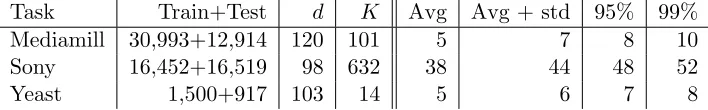
Task Train+Test d K Avg Avg + std 95% 99% Mediamill 30,993+12,914 120 101 5 7 8 10 Sony 16,452+16,519 98 632 38 44 48 52 Yeast 1,500+917 103 14 5 6 7 8

Table 1: Main statistics related to the three data sets used in our experiments. The last four columns give information on the distribution of the number of labels per instance. “Avg” denotes the (rounded) average number of labels over the training examples, and “Avg+std” gives the average augmented by one unit of standard deviation. So, for instance, in the Mediamill data set, the average number of labels per instance in the training set is 5, with a standard deviation of 2. The columns tagged “95%” and “99%” give an idea of the quantiles of this distribution. E.g., on Mediamill, 95% of the training examples have at most 8 classes (out of 101), on the Sony data set, 99% of the training examples have at most 52 classes (out of 632).

5. Experiments

The experiments we report here are meant to validate the exploration-exploitation tradeoff implemented by our algorithm along different axes: data set size, label set size, loss function, label generation model, training mode of operation, and restrictions on the total number of classes predicted. Moreover, we explicitly tested the effectiveness of ranking classes based on upper confidence-corrected probability estimates.

5.1 Data Sets

We used three diverse multilabel data sets, intended to represent different real-world condi-tions. The first one, called Mediamill, was introduced in a video annotation challenge (Snoek et al., 2006). It comprises 30,993 training samples and 12,914 test ones. The number of features d is 120, and the number of classes K is 101. The second data set is the music annotated Sony CSL Paris data set (Pachet and Roy, 2009), made up of 16,452 training samples and 16,519 test samples, each sample being described by d = 98 features. The number of classesK is 632, which is significantly larger than Mediamill’s. The third one is the smaller Yeast data set (Elisseeff and Weston, 2002), made up of 1,500 training samples, 917 test samples, with d = 103 and K = 14. In all cases, the feature vectors have been normalized to unit Euclidean norm. Table 1 summarizes relevant statistics about these data sets. This table also gives an idea of the distribution of the number of classes per instance.

5.2 Parameter Setting and Loss Measures

For the practical implementation of the algorithm in Figure 2, we simplified the formula for 2_i,t. This is justified by the fact that the actual constants in the definition of 2_i,t are artifacts of our high-probability upper bounds. Hence, we used

(19)

whereα is a parameter that we found by cross-validation on each data set across the range α = 2−8,2−7, . . . ,27,28, for each choice of the label-generation model, loss setting, and value of S—see below. We have considered two different loss functions L, the square loss and the logistic loss (denoted by “Log Loss” in our plots). Correspondingly, the two label-generation models we tested are the linear model Pt(yi,t = 1) = (1 +u>i xt)/2 with domain

D= [−1,1], and the logistic modelPt(yi,t = 1) =eu >

ixt/(eu>ixt+ 1). In the logistic case, it

makes sense in practice not to place any restrictions on the margin domainD, so that we set R=∞. Again, because our upper bounding analysis would yield as a consequencec00_L= 0, we instead setc00_Lto a small positive constant, specificallyc00_L= 0.1, with no special attention to its fine-tuning. The setting of the cost functionc(i, s) depends on the task at hand, and we decided to evaluate two possible settings. The first one, denoted by “decreasing” is c(i, s) = s−i_s+1, i = 1, . . . , s, the second one, denoted by “constant”, is c(i, s) = 1, for all i and s. In all experiments with `a,c, the a parameter was set to 0.5 (so that `a,c with

constant c reduces to half the Hamming loss). In the decreasing c scenario, we evaluated the performance of the algorithm on the loss`a,c that the algorithm is minimizing, but also

its ability to produce meaningful (partial) rankings through `p−rank,t. In the constant c

scenario, we only evaluated the Hamming loss, its natural loss function.

As is typical of multilabel problems, the label density of our data sets, i.e., the average fraction of labels associated with the examples, is quite small. Hence, it is clearly beneficial to our learning algorithm to bias its inference process so as to produce short ranked lists

ˆ

Yt. We did so by imposing, for all t, an upper boundSt=S on |Yˆt|. For each of the three

data sets, we tried out the four different values of S reported in the last four columns of Table 1: the average number of labels; the average plus one standard deviation, the number of labels that covers 95% of the examples, and the number of labels that covers 99% of the examples, all figures only referring to the corresponding training sets.

5.3 Baselines

As a baseline, we considered a full information version of Algorithm 2, denoted by “Full Info”, that receives after each prediction the full array of true labels Yt for each

sam-ple. Comparing to full information algorithms stresses the effectiveness of the explo-ration/exploitation rule above and beyond the details of underlying generalized linear pre-dictor. We also compared against the random predictor (denoted by “Random”) that simply outputs at timeta ranked list ˆYt made up of S labels chosen (and ranked) at random.

Fi-nally, an interesting ranking baseline which targets the ranking ability of our algorithm is one that lets our partial feedback algorithm select which classes to include in ˆYt, and then

shuffles them at random within ˆYt to produce the ranked list. This baseline we only used

with the ranking loss`p−rank,t, and is denoted by “Shuffled” in our plots.

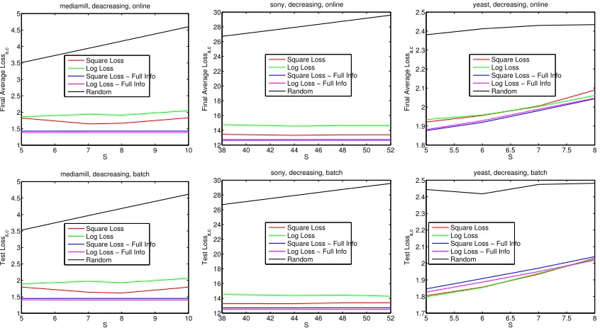
5.4 Results

(20)

The plots report online or batch loss measures as a function of S,11 averaged over 5 random permutation of the training sequence. Specifically, whereas the online measure of performance (“Final Average ... Loss”) is the cumulative loss accumulated during training, divided by the number of samples in the training set, the batch measure (“Test ...”) is simply the average loss over the test set achieved by the last solution produced by train-ing. For the partial-feedback algorithms (“Square Loss”, “Log Loss” and, in the ranking case, also “Square Loss Shuffled” and ”Log Loss Shuffled”), only the bestα-cross-validated performances are shown. Moreover, in the ranking experiments, because of the explicit de-pendence of`p−rank,t onS, we instead considered the scaled version of the loss `p−rank,t/S.

Notice that the theoretical results contained in Section 4 still apply to this scaled loss function.

The first thing to observe from the evidence we collected is that performance in the batch setting closely follows the one in the online setting, across all the data sets, conditions and losses. In a sense, this is to be expected, since the order of samples in the training set is randomly shuffled.

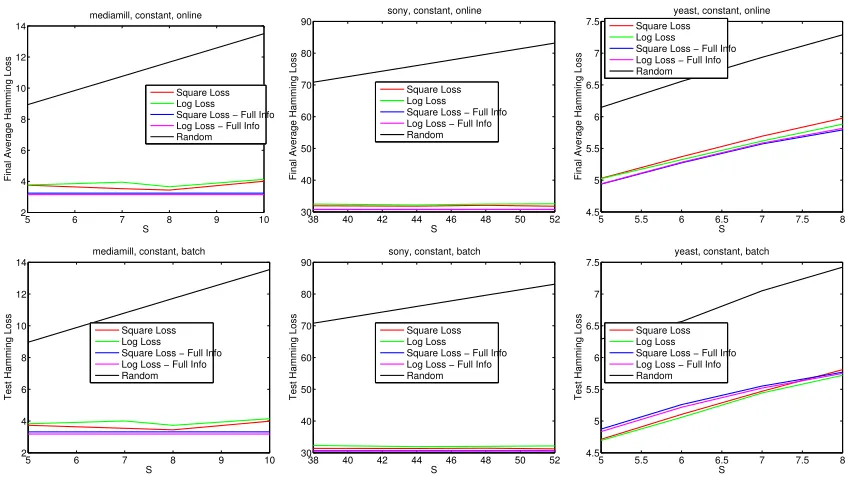
The optimal value of S that allows us to best balance exploration and the exploitation of the algorithm seems to be depending on the particular data set and task at hand. So, for instance, on Mediamill with Hamming loss, this value isS = 8, corresponding to the 95% coverage of the training set, while on Yeast it is the average value S = 5, covering around 50% of the training examples. When the loss is `a,c, the best value of S clearly depends

on the costs c. In the ranking case, performance increases as S gets larger, but this is very likely to be due to the scaling factor 1/S in the loss we plotted. Notice that, from our theoretical analysis in Section 3, the algorithm (e.g., in the special case on Hamming loss) should in principle be able to determine the best size of ˆYt at each round, so that setting

St = K for all t is still a fair choice. Yet, this conservative setting makes the algorithm

face an unnecessarily large action space (of sizeK!), and correspondingly a harder inference problem, rather than the substantially smaller space (of sizeK(K−1)(K−2). . .(K−S+1)) obtained by settingSt=S. This is evinced by the fact that all plots (regarding both partial

and full information algorithms) in Figure 4 tend to be increasing with S. For the very sake of this inference, the fact that all algorithms see the examples only once seems to be a severe limitation.12

The performance of our partial information algorithms are always pretty close to those of the corresponding full information algorithms. This empirically validates the explo-ration/exploitation scheme we used. Also, in all cases, all algorithms clearly outperform the random predictor. In most of the experiments, the linear model (“Square Loss”) seems to deliver slightly better results in the bandit setting than the logistic model (“Log Loss”), while the performance of the two models is very similar in the full information case. Ex-ceptions are the constant and the decreasing cost settings in the batch case on the Yeast data set (Figure 3, bottom right, and Figure 4, bottom right), where the bandit algorithm has an even better performance than the full information one. This is perhaps due to the

11. The plots are actually piecewise linear interpolations with knots corresponding to the 4 values of S

mentioned in the main text.

12. Training for a single epoch is a restriction needed to carry out a fair comparison between full and

(21)

5 6 7 8 9 10 1 1.5 2 2.5 3 3.5 4 4.5 5

mediamill, deacreasing, online

S

Final Average Loss

a,c

Square Loss Log Loss Square Loss − Full Info Log Loss − Full Info Random

38 40 42 44 46 48 50 52 12 14 16 18 20 22 24 26 28 30

sony, decreasing, online

S

Final Average Loss

a,c

5 5.5 6 6.5 7 7.5 8

1.8 1.9 2 2.1 2.2 2.3 2.4 2.5

yeast, decreasing, online

S

Final Average Loss

a,c

5 6 7 8 9 10

1 1.5 2 2.5 3 3.5 4 4.5 5 S Test Loss a,c

mediamill, deacreasing, batch

38 40 42 44 46 48 50 52

12 14 16 18 20 22 24 26 28 30 S Test Loss a,c

sony, decreasing, batch

5 5.5 6 6.5 7 7.5 8

1.7 1.8 1.9 2 2.1 2.2 2.3 2.4 2.5 S Test Loss a,c

yeast, decreasing, batch

Figure 3: Experiments with `a,c and decreasing costs.

noise introduced during exploration, that acts as a kind of regularization, improving gener-alization performance in such a small data set. In general, however, the comparison linear vs. logistic is somewhat mixed.

In the ranking setting (Figure 5) we also show the performance of our algorithm when the order of predicted labels is randomly permuted (“Shuffled”). It is shown that, uniformly over all settings, shuffling causes performance degradation, thereby proving that our algorithm is indeed learning a meaningful ranking over the labels in the set ˆYt, even without receiving

any ranking feedback within this set from the user.

6. Technical Details

This section contains all proofs missing from the main text, along with ancillary results and comments.

The algorithm in Figure 2 works by updating through the gradients ∇i,t of a modular

margin-based loss function PK_i₌₁L(w>_i x) associated with the label generation model (2), i.e., associated with functiong, so as to make the parameters (u1, . . . ,uK) ∈ RdK therein

achieve the Bayes optimality condition

(u1, . . . ,uK) = arg min w1,...,wK:w>

i xt∈D Et

" _K X

i=1

L(si,tw>i xt) #

, (6)

whereEt[·] above is over the generation ofYt in producing the sign valuesi,t ∈ {−1,0,+1},

conditioned on the past (in particular, conditioned on ˆYt). The requirement in (6) is akin

(22)

5 6 7 8 9 10 2 4 6 8 10 12 14 S

Final Average Hamming Loss

mediamill, constant, online

38 40 42 44 46 48 50 52

30 40 50 60 70 80 90 S

sony, constant, online

5 5.5 6 6.5 7 7.5 8 4.5 5 5.5 6 6.5 7 7.5 S

yeast, constant, online Square Loss

Log Loss Square Loss − Full Info Log Loss − Full Info Random

5 6 7 8 9 10

2 4 6 8 10 12 14 S

Test Hamming Loss

mediamill, constant, batch

38 40 42 44 46 48 50 52

30 40 50 60 70 80 90 S

Test Hamming Loss

sony, constant, batch

5 5.5 6 6.5 7 7.5 8

4.5 5 5.5 6 6.5 7 7.5 S

Test Hamming Loss

yeast, constant, batch

Figure 4: Experiments with`a,c and constant costs (Hamming loss).

The above is combined with the ability of the algorithm to guarantee the high probability convergence of the prototype vectorsw0_i,t to the correspondingui (Lemma 13). The rate of

convergence is ruled by the fact that the associated upper confidence values i,t shrink to

zero as √1

t whentgrows large. In order for this convergence to take place, it is important to

insure that the algorithm is observing informative feedback (either “correct”, i.e., si,t = 1,

or “mistaken”, i.e., si,t = −1) for each class i contained in the selected ˆYt. This in turn

implies regret bounds for both `a,c (Lemma 11) and `p−rank,t (Lemma 12).

The following lemma faces the problem of hand-crafting a convenient loss function L(·) such that (6) holds.

Lemma 9 Letw1, . . . ,wK ∈ RdK be arbitrary weight vectors such thatwi>xt∈D,i∈[K],

(u1, . . . ,uK) ∈ RdK be defined in (2), si,t be the updating signs computed by the algorithm

at the end (Step 5) of time t, L : D= [−R, R]⊆ R → R+ _{be a convex and differentiable}

function of its argument, with g(∆) =−L0(∆). Then for any t we have

Et " _K

X

i=1

L(si,tw>i xt) #

≥_E_t

"_K

X

i=1

L(si,tu>i xt) #

,

i.e., (6) holds.

Proof Let us introduce the shorthands ∆i = u>i xt, ∆b_i = w>_i,tx_t, s_i = s_i,t, and p_i = P(yi,t = 1|xt) = L

0_(−∆

i) L0_(∆

i)+L0(−∆i) =

g(−∆i)

g(∆i)+g(−∆i). Moreover, let Pt(·) be an abbreviation

(23)

5 6 7 8 9 10 1 1.5 2 2.5 3 3.5 4 4.5

mediamill − decreasing, online

S

Final Average Ranking Loss/S

Square Loss Square Loss Shuffled Log Loss Log Loss Shuffled Random Square Loss − Full Info Log Loss − Full Info

38 40 42 44 46 48 50 52

15 20 25 30 35 40

sony − decreasing, online

S

5 5.5 6 6.5 7 7.5 8

1.8 2 2.2 2.4 2.6 2.8 3 3.2

yeast − decreasing, online

S

5 6 7 8 9 10

1 1.5 2 2.5 3 3.5 4 4.5

mediamill − decreasing, batch

S

Test Ranking Loss/S

38 40 42 44 46 48 50 52

15 20 25 30 35 40

sony − decreasing, batch

S

Test Ranking Loss/S

5 5.5 6 6.5 7 7.5 8

1.8 2 2.2 2.4 2.6 2.8 3 3.2 3.4 3.6

yeast − decreasing, batch

S

Test Ranking Loss/S

Figure 5: Experiments with the ranking loss `p−rank,t. In order to obtain

“scale-independent” results, in this figure we actually used `p−rank,t/S rather than

`p−rank,titself.

constructed (Figure 2), we can write

Et "_K

X

i=1

L(si,t∆b_i) #

=X

i∈_Ytˆ

Pt(si,t = 1)L(∆b_i) +_P_t(s_i,t=−1)L(−∆b_i)

+ (K− |Yˆt|)L(0)

=X

i∈_Ytˆ

piL(∆b_i) + (1−p_i)L(−∆b_i)

+ (K− |Yˆt|)L(0),

For similar reasons,

Et "_K

X

i=1

L(si,t∆i) #

=X

i∈_Ytˆ

(piL(∆i) + (1−pi)L(−∆i)) + (K− |Yˆt|)L(0).

Since L(·) is convex, so is Et h

PK

i=1L(si,t∆b_i) i

when viewed as a function of the ∆b_i. We

have that ∂Et[

PK

i=1L(si,t∆b_i)]

∂∆bi = 0 if and only if for all i

∈Yˆt we have that∆bi satisfies

pi =

L0(−∆b_i)

L0(∆b_i) +L0(−∆b_i)

.

Sincepi = L

0_(−∆

i) L0_(∆

i)+L0(−∆i), we have thatEt h

PK

i=1L(si,t∆b_i) i

is minimized when∆b_i = ∆_ifor

(24)

Let now V art(·) be a shorthand forV ar(· |(y1,x1), . . . ,(yt−1,xt−1),xt). The following

lemma shows that under additional assumptions on the lossL(·), we can bound the variance of a difference of lossesL(·) by the expectation of this difference. This will be key to proving the fast rates of convergence contained in the subsequent Lemma 13.

Lemma 10 Let (w0₁_,t, . . . ,w0_K,t) ∈ RdK _{be the weight vectors computed by the algorithm}

in Figure 2 at the beginning (Step 2) of time t, si,t be the updating signs computed at the

end (Step 5) of time t, and (u1, . . . ,uK)∈ RdK be the comparison vectors defined through

(2). Let L : D = [−R, R]⊆ R → R+ _{be a} _C2₍_D₎ _{convex function of its argument, with}

g(∆) = −L0(∆) and such that there are positive constants c0_L and c00_L with (L0(∆))2 ≤ c0_L

and L00(∆)≥c00_L for all ∆∈D. Then for any i∈Yˆt

0≤V art

L(si,tx>tw0i,t)−L(si,tu>i xt)

≤ 2c

0

L

c00_L Et

h

L(si,tx>tw0i,t)−L(si,tu>i xt) i

.

Proof Let us introduce the shorthands ∆i = x>tui, ∆b_i = x>_tw0_i,t, s_i = s_i,t, and p_i = P(yi,t = 1|xt) = L

0_(−∆

i) L0_(∆

i)+L0(−∆i) =

g(−∆i)

g(∆i)+g(−∆i). Then, for any i∈[K],

V art

L(si,tx>t w

0

i,t)−L(si,tu>i xt)

≤Et

L(si∆b_i)−L(s_i∆_i)

2

≤c0_L(∆b_i−∆_i)2. (7)

Moreover, for anyi∈Yˆtwe can write

Et h

L(si∆b_i)−L(s_i∆_i) i

=pi(L(∆b_i)−L(∆_i)) + (1−p_i) (L(−∆b_i)−L(−∆_i))

≥pi

L0(∆i)(∆b_i−∆_i) +

c00_L

2 (∆bi−∆i) 2

+ (1−pi)

L0(−∆i)(∆i−∆) +b

c00_L

2 (∆bi−∆i) 2

=pi

c00_L

2 (∆bi−∆i)

2_{+ (1}₋_p

i)

c00_L

2 (∆bi−∆i) 2 = c

00

L

2 (∆bi−∆i)

2_, ₍₈₎

where the second equality uses the definition ofpi. Combining (7) with (8) gives the desired

bound.

We continue by showing a one-step regret bound for our original loss`a,c. The precise

connection to loss L(·) will be established with the help of a later lemma (Lemma 13).

Lemma 11 Let L : D = [−R, R] ⊆ R → R+ _{be a convex, twice differentiable, and}

nonincreasing function of its argument. Let (u1, . . . ,uK) ∈ RdK be defined in (2) with

g(∆) =−L0(∆) for all∆∈D. Let also cL be a positive constant such that

L0(∆)L00(−∆) +L00(∆)L0(−∆)