http://www.sciencepublishinggroup.com/j/pamj doi: 10.11648/j.pamj.20170602.13
ISSN: 2326-9790 (Print); ISSN: 2326-9812 (Online)
Shallow Water 1D Model for Pollution River Study
Antoine Celestin Kengni Jotsa
1, *, Vincenzo Angelo Pennati
2, Antonio Di Guardo
2, Melissa Morselli
21Department of Fundamental Sciences, Laws and Humanities, Institute of Mines and Petroleum Industries, University of Maroua at Kaéle,
Maroua, Cameroon
2Science and High Tecnology Department, Università Degli Studi Dell'Insubria, Via Valleggio, Como, Italy
Email address:
antoinekengni@yahoo.fr (A. C. K. Jotsa), vpennati@teletu.it (V. A. Pennati), antonio.diguardo@uninsubria.it (A. D. Guardo), melissa.morselli@uninsubria.it (M. Morselli)
*Corresponding author
To cite this article:
Antoine C. Kengni Jotsa, Vincenzo A. Pennati, Antonio Di Guardo, Melissa Morselli. Shallow Water 1D Model for Pollution River Study.
Pure and Applied Mathematics Journal. Vol. 6, No. 2, 2017, pp. 76-88. doi: 10.11648/j.pamj.20170602.13 Received: February 25, 2017; Accepted: March 23, 2017; Published: April 15, 2017
Abstract:
In this paper a finite element 1D model for shallow water flows with distribution of chemical substances is presented. The deterministic model, based on unsteady flow and convection-diffusion-decay of the pollutants, allows for evaluating in any point of the space-time domain the concentration values of the chemical compounds. The numerical approach followed is computationally cost-effectiveness respect both the stability and the accuracy, and by means of it is possible to foresee the evolution of the concentrations.Keywords:
Partial Differential Equation, Finite Elements, Shallow Water Flow, River Pollution1. Introduction
When considering river flows with an essential lack of transversal velocity component, the obvious choice to calculate the discharge and the pollutant concentrations is to use a 1D shallow water (SW) model. One dimensional schemes are still a practical tool for modeling river flows, in particular for simulations over extended time [23]. For flow essentially 2D, of course, a fully 2D shallow water model should be considered [2]. In literature, exists a large amount of numerical models used for the solution of the systems of partial differential equations, they are traditionally based on finite element, finite difference or finite volume approximations in space and on implicit or explicit schemes in time [1]. We adopt for the solution of the SW system a fractional step scheme in time and a finite element (FE) approximation in space [2, 15]. In particular, the choice of the fractional step afford, at every time step, to decouple the physical contributions so that waves traveling at speed of √gh
can be calculated implicitly, with a low computational cost. In order to save computational time, moreover, the non-linear part of the momentum equation (and also the total derivative of the chemical pollutant transport equations) is solved using the characteristics method, so that the most onerous
flow and three convection-diffusion equations and decay lows (without air and sediments interactions) for the pollutant concentrations.
The remainder part of the paper is organized as follows: in the next section the numerical model is presented in detail; then follows two sections reporting two numerical tests with known analytical solution; in the fourth section an application to a real problem is presented (the Novella river problem) reporting the results of a transient of 28 hours occurred in the autumn of 2009; finally some conclusions are drawn in the last section.
2. Mathematical and Numerical Model
2.1. Governing Equations
To develop the numerical model, we start from the 1D classical shallow water equations represented by the Saint-Venant system, it is formed by the momentum equation (with dependent variable the unit width discharge q) and by the water height h equation (in our formulation replaced by the elevation ξ of the free surface respect to a reference level). The 1D approach presented here is suitable for situations in which the river presents an almost constant width and meanders are absent, it is based on the assumptions of constant flow in the vertical direction and hydro-static pressure. The Saint-Venant system of partial differential equations, in conservative form reads:
+ − + ℎ + = (1)
+ = 0 (2) and the transport and decay equations for concentrations read:
+ − + , = , , ! (3)
= " − # , = , , ! (4)
where: x is the spatial coordinate, t is the time, h(x,t) is the total depth water measured from the bottom of the river,
q(x,t) is the unit width discharge, u(x,t)=q(x,t)/h(x,t) is the velocity, ξ(x,t) is the elevation over the reference plane,
f(x,t) is the source term, g is the gravitational acceleration, µ
is the diffusion coefficient, α is the bottom slope of the river. Marking by i in turn P, D, M, ai(x,t) is the reaction
function, ci(x,t) is the concentration of the pollutant, si(x,t)
is the source term for transport equation, Γi is the diffusion
coefficient, Si(x,t) is the source term for decay equation and ri is a decay ratio. We recall that (1) represents the
conservation of the momentum, while (2) ensure the conservation of mass, (3) is the convection dominated transport of the pollutants along the river and, finally, (4) keeps into account the decay effects.
Suitable initial and boundary conditions have to be added in order to make the overall system solvable.
2.2. Numerical Scheme
Some features of the numerical approach developed have to be remarked, in fact the non-linear convective term of momentum equation is approximated by the characteristics method, so that the spurious oscillations due to centered approximations are avoided under mild restrictions on the time step and, moreover, a fractional step procedure is adopted for advancing in time. This last choice is made in order to decouple, at every time step, the physical contributions [5] obtaining the important advantage that the critical time step is in term of the flow velocity instead of the wave celerity. The spatial discretization of the equations is based on a Galerkin FE method, with two different spaces for the unknowns: polynomials of degree two for the unit width discharge and concentrations, polynomials of degree one for the elevation. It is notable to underline that the following advantages are guaranteed from our FE choice: the possibility to use h-adaptive techniques (used in this paper for the solution of the second numerical test), the absence of numerical viscosity inherent to the low order interpolation at the foot of characteristics and the elimination of the spurious oscillations that can arise when an equal order approximation is used [26]. Let Ω a domain in R and [0, T] the time interval of study. In detail, the fractional step we use for advancing in time is:
un = qn/hn, hn = h0+ξn (5)
$% &' = $()
*) with )*= ) − +, $()-)
and
)- = ) − /0 $()) (6)
(xf is the foot of characteristic relevant to the node with
abscissa x)
1$% &' = ℎ$ $% ' & (7)
1$%02 = 1$%32 − ∆, ℎ$+ ∆, 501$%32
5)0 + $%02
with
$% ' = ∆, 67 ' 67 &'
( 6)8/': (8) (f represents the bottom friction, it depends on the Strickler parameter K)
;$%3 − (+,)0 5
5) < ℎ$5;
$%3
5) = + +,5) >5 1
$%02
ℎ$ ;$%3? =
;$− +, 67'+ +, < 67'
equation:
1$%3− 1$% 02+ ∆, ℎ$5;$%3
5)
+ 67'6 (;$%3− ;$) = 0 (10)
and subtracting the result to the equation:
;$%3− ;$+ +, 67& = 0 (11)
1$%3= 1$% 02− +, ℎ$5; $%3
5)
+ 67'6 (;$%3− ;$) = 0 (12)
$%3 = 67&
67&and ℎ$%3= ℎ@+ ;$%3 (13) )*A= ) − +, $%3()-)
and
)- = ) − /0 $%3()) (14)
(xfa indicates the adjourned value of the characteristic foot)
67&B6( CD)
∆ − Γ
67&
= 0, = , , ! (15)
̃$%3 = # $%3, = , , ! (16)
where ri = r
i ∆t and ai,, si,, Si are null.
Remark 2.2.1.Equations (15) and (16) make completed the phenomenon of convection, diffusion and decay.
Remark 2.2.2. The use of characteristics for the approximation of the convective terms (both for the momentum equation and for the transport equations of chemical substances) requires an interpolation of high order; this is easily obtained because of our P2 choice for qand ci
variables (we recall that we use P1 elements only for ξ
variable).
2.3. Algebraic Formulation
Since the spatial approximation is based on Galerkin FE method, the algebraic formulation reads:
for the provisional discharge qn+2/3, indicating by
MLq the lumped mass matrix, by Aq the stiffness matrix, by G1 the diagonal matrix with g1i,i=1-∆tg(qn+1/3)i/(hn)i7/3K2:
G3HIJK$%'= HIJK$%
&
' − ∆, HIJL$ − ∆, M K$%&' (17) For the elevation ξn+1, indicating by
ML and by A the lumped mass matrix and stiffness matrix respectively, by BT
the matrix of the integral of the product between the basis function and its derivative, by G2 the diagonal matrix with
g2i,i=g(hn)i, by G3 the diagonal matrix with g3i,i= (qn+2/3)i/(hn)i:
[HI + (∆,)0G0 M + ∆, G2OP]R$%3 =
HIR$ + ∆,G2OPR$− ∆,OP K$%' (18)
Remark 2.3.1. In equation (18), the q values considered are those associated with the boundary nodes of the elements.
For the update value of the qn+1 discharge, indicating by
MLq the lumped mass matrix of discharge, by CT the matrix of the integral of the product between the basis function and its derivative, by G2 and G3 the above defined diagonal matrices:
HIJK$%3 = HIJK$%02− ∆,G0SPR$%3
+G2HIJ(R$%3− R$) (19)
Remark 2.3.2. In (19), the ξ values considered are those calculated in the boundary nodes and in the middle node of each element.
For the chemical pollutant ci, indicating by
MLci the lumped mass matrix and by Aci the stiffness matrix:
[HITU+ ∆, Γ MTU] $%3 = H
I TU $()
*A) (20)
Remark 2.3.3. The matrices Aq, and MLq, are equal to the matrices Aci and MLci respectively. Thus the only matrices we have to construct are: Aq, A, MLq, ML, B, and C.
Remark 2.3.4. We would stress that in the approach over presented, the only systems we have to solve are of elliptic kind and are relevant only to the ξ and civariables.
Remark 2.3.5. Since the matrix of the system (18) is tri-diagonal, the Thomas algorithm has been used for its solution, while the Schwarz preconditioned iterative Bi-CGSTAB solver has been used for the systems of (20). In the next section a short presentation of the Schwarz preconditioner is presented.
2.4. Schwarz Scalable Additive Preconditioner
We give a brief description of the Schwarz preconditioner for elliptic problems introduced in [21] and adopted in this paper. In order to fix the ideas, we refer to a Poisson problem with homogeneous boundary conditions:
-∆u = f in Ω and u = 0 on ∂Ω (21)
The FE approximation to the Poisson problem consists in finding uh∈ Vh ⊂ V = H01(Ω) such that ah (uh,vh) = (f, vh)
with ah(·,·) the bi-linear form given by ah (uh,vh) = ∫Ω
∇
uh*∇
vh dΩ and (f, vh) is the linear form defined as (f, vh) = ∫Ω f *vh dΩ.If we consider, for example, the domain as decomposed in two overlapping sub-domains Ω1and Ω2, let be ∂Ω, ∂Ω1, ∂Ω2
the boundaries of Ω, Ω1, Ω2 respectively, and Γ1, Γ2 the
internal boundaries of Ω1, Ω2 respectively. The Schwarz
approach consists of defining two sequences u1k+1 and u2k+1
with k ≥ 0, and solving iteratively the two boundary-value problems:
-∆u1k+1= f in Ω1
u1k+1 = 0 on ∂Ω U ∂Ω1 and u1k+1 = u2k on Γ1 (22)
and
-∆u2k+1= f in Ω2
with
u2k+1 = 0 on ∂Ω U ∂Ω2 and u2k+1 = u1k on Γ2 (23)
For the algebraic formulation of the Schwarz method one can think that the domain Ω is subdivided by M sub-domains Ωiwith i = 1,…, M. We define the prolongation operator RiT, that extends by zeros the degree of freedom outside Ωi, and the restriction operator Ri like its transposed. By denoting Ah
and Ai the stiffness matrices with respect to the global and
local bi-linear forms ah (·, ·) and ai (·, ·) and defining the
operator Qilike the matrix Qi= RiTAi-1Ri, then after some algebraic manipulations the one level additive Schwarz iterative method reads for M ≥ 2 sub-domains:
uhk+1 = uhk + (∑iQi)(bh - Ahuhk) (24) with k ≥ 0 index of iteration. Regarding (24) as a fixed-point relation, we can define the Schwarz method simply as a Richardson iterative method with preconditioner Pas-1 = [Σi
Qi]. Unfortunately, the convergence of the one level Schwarz
method deteriorates when the number M of sub-domains becomes larger because of the lack of information between sub-domains Ωi. In order to overcome this drawback, we
introduce a global coarse mesh as a particular sub-domain Ω1, so that communications among all the sub-domains are
guaranteed. Therefore, the final form of the preconditioner is
Pasc-1= [Σi Qi] with i = 1, …, M. Since the algebraic system
of (21) is Ahuh = bh, the preconditioned two level additive Schwarz system becomes:
(ΣiRiTAi-1Ri) Ahuh = (ΣiRiTAi-1Ri) bh (25)
Remark 2.4.1. The number M of the sub-domains in which Ω is divided, decides the efficiency of the Schwarz preconditioner. In fact, the number of nodes belonging to each sub-domain depends on M and also on the sub-domains length; both the choices should be as shrewd as possible in order to reach a good balance among the dimension of the local stiffness matrices Ai and the optimal computational time. Another choice influences the efficiency of the Pasand
Pascpreconditioners, namely the level of fill-in allowed in the
process of LU factorization to calculate the matrices Ai-1, the
so-called Incomplete LU factorization (ILU) process. The algorithm of the implementation of the Schwarz scalable additive preconditioner can be seen in [15].
2.5. Numerical Procedure
In summary, the fractional step works following these steps:
1) The unit width discharge qn, the depth hn, the elevation
ξ n and the concentrations ci n are given at time t = tn
2) Compute the velocity unby (5) 3) Compute the velocity un+1/3 by (6)
4) Compute the unit width discharge qn+1/3by (7)
5) Compute the unit width discharge qn+2/3by (17)
6) Compute the adjourned value of the elevation ξ n+1 by
(18)
7) Compute the adjourned value of the unit width discharge qn+1 by (19)
8) Compute the adjourned values of velocity un+1 and
depth hn+1 by (13)
9) Compute the adjourned value of concentrations ci n+1
using (20)
10)Compute the corrected concentrations by (16)
11)Go to 1 and repeat the above procedure until the desired solution is obtained.
3.
Numerical Test with Analytical
Solution
The correctness and efficiency of the developed model have been checked solving the following problem with analytical solution. In fact, the expression of the elevation and the discharge, similar to that of [25], are the following:
;(), ,) = 0.2 sin(3800 )) cos(2\ 3800 ,)2\
1(), ,) = 0.9 − 0.2 cos(3800 )) sin(2\ 3800 ,)2\
ℎ(), ,) = 3 + ;(), ,) (26) giving rise to the source function:
(), ,) = 5.686def − 0.3924def0 + @.2hijk
2%@.0jl− @.@mijk
2%@.0jl −[@.0inl][@.oB@.0nk](2%@.0jl) (27)
where:
A =3800 , e = cos(d)), f cos(d,)2\
= sin(d)) , q = sin(d,) (28) Two analytical solutions were also taken for the concentrations:
3(), ,) = 1 + sin 2m@@st ) cos 2m@@st , (29)
0(), ,) = 1 − cos 2m@@st ) sin 2m@@st , (30)
therefore the source functions for the concentrations were respectively:
3(), ,) = −u sin(u)) sin(u,) + u cos(u)) cos(u,) +
Γ3u0sin(u)) cos(u,) + 3(1 + sin(u)) cos(u,)) (31)
0(), ,) = −u cos(u)) cos(u,) + u sin(u)) sin(u,) −
with u=q/h and F=4π/3800
For the analytical test we fixed α=0; moreover we choose
µ=0, g=9.81, Γ1 =Γ2 =0.001, a1=0.0000174, a2=0.0115 and
did not take into account decay effects. The domain considered was Ω=[0, 3800], partitioned in 950 elements of equal length; the number of nodes was 1901 for the discharge
q and the pollutants c1 and c2; 951 for the elevation ξ. The
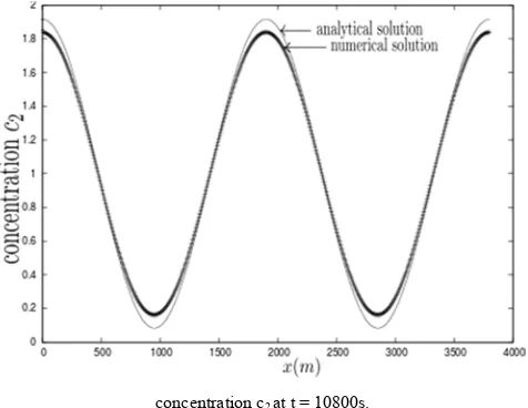
transient studied was 10800 s and ∆t=100 s. The initial and boundary conditions were obtained by the analytical solutions and we imposed Dirichlet at inflow and Neumann at outflow for ξ, c1 and c2; while we imposed only Dirichlet
at inflow for q. In figure 1 we report the distribution of analytical and numerical solutions of concentration c2 at time 10800 s and in figure 2 the time evolution of analytical and numerical solutions of concentration c2 at node 238 (x=237).
For the other results and comments, we refers to [14].
concentration c2 at t = 10800s.
Figure 1. Distribution of analytical and numerical c2 values.
concentration c2 at node 238 (x= 237).
Figure 2. Time evolution of analytical and numerical c2 values.
4. Sub-Critic Flow in a Channel
In order to solve problems defined in channels with variating cross section the equations (1) and (2) have to be updated:
2
2 f
f f
Q+ QQ Q+ gA α + h = f
A
t x A x x
µ ∂ ∂ ∂ ∂ −
∂ ∂ ∂ ∂ (33)
1 0
f
ξ Q
+ B =
t x
∂ ∂
∂ ∂ (34)
with Q total discharge, h depth of water, Af and Bf cross
section and width channel respectively. Following the fractional step seen in the section 2, the modified algebraic system reads:
given at tn: Qn, A
fn, Bfn, hn= h0+ξn, un=Qn/Afn, un+1/3=un(x
f) with xf=x-∆tun(xI) and xI=x-(∆t/2)un(x) (35) Qn+1/3 = A
fn un+1/3 (36)
Indicating by ML the lumped mass matrix, by A the stiffness matrix, by H1 the diagonal matrix with h1i,i =1-∆tgM2(Qn+1/3)
i/(Afn)i(Rn)4/3i, with M and R Manning
coefficient and hydraulic radius respectively, by H2 the diagonal matrix with h2i,i=1/(Afn)i:
v3HIw$% 02= HIw$% 32 −
∆, HIx*$ ∆, v
0Mw $% &
' (37)
For the elevation ξn+1, indicating by M
L and by A the lumped mass matrix and stiffness matrix respectively, by CT
the matrix of the integral of the product between the basis function and its derivative, by G2 the diagonal matrix with
g2i,i=g(hn)i, by H3 the diagonal matrix with h3i,i= (Qn+2/3)
i/(Afn)i, by H4 the diagonal matrix with h4i,i= 1/(Bfn)i:
NHI (∆,.0G0M ∆,v2SPQR$%3
HIR$ ∆,v2SPR$ ∆,vsSPw$% ' (38)
For the update value of the Qn+1 discharge, indicating by
ML the lumped mass matrix of discharge, by CT the matrix of the integral of the product between the basis function and its derivative, by H5 the diagonal matrix with h5i,i= g(Afn)i, and
H6 the diagonal matrix with h6i,i= (Qn+2/3)i/(hn)i:
HIw$%3 HIw$% 0
2 ∆,vySPR$%3
vh HI(R$%3 R$. (39)
By means of the above method we solve the steady problem reported in [8, 12]. The domain is Ω=[0, 3], the height is h = 1-zb-ξ0,with ξ0asfigure 3, and bottom zb as:
(
)
2
0 1cos 1 5 1 5 0 5
0
b
. πx . π for x - . .
z
otherwise
− ≤
=
(40)
The channel width is given by:
(
)
2
1 0 1cos 1 5 1 5 0 5
1 0
f
. πx . π for x - . .
B
. otherwise
− − ≤
=
The boundary conditions imposed are Q=0.1 m3/s at inflow (x=0) and water height h=1.0 at outflow (x=3.0), that cause a subcritical flow over the whole domain. The spatial discretization consists of 230 FE respecting an h-adaptive
criterion, in fact in the intervals [0; 0.1], [0.8; 2.2] and [2.9; 3]
∆x=0.01, while in the intervals [0.1; 0.8] and [2.2; 2.9]
∆x=0.02. The basis functions are second degree polynomials for both ξ and Q. The steady state was obtained simulating a transient of 25000 time steps; keeping into account the properties of equation (38) and in order to save computational time, we use two different time intervals for Q and ξ, that is
∆t1=0.0002 for Q and ∆t2=0.005 for ξ. The system (38) was solved by means of Bi-CGSTAB iterative solver, with about 60 iterations for each time step. For this test we don’t use preconditioning and the iterations are stopped when dif < ε,
with dif=difference of two consecutive iterations and ε = 10-12.
In figures 3 and 4 are reported the graphics of analytical and numerical solutions for ξ and Q respectively and in figures 5 and 6 are indicated the time history of the errors relevant to ξ
and Q respectively. The maximum differences err between the analytical and numerical solution, at the end of the transient, are: for the elevation ξ,err = 3.04*10-5 and for the discharge
Q, err = 4.73*10-6.
Figure 3. Analytical and numerical elevation ξ (dashed and bold line respectively).
Figure 4. Analytical and Numerical discharge Q (dashed and bold line respectively).
Figure 5. Time history of error elevation ξ.
Figure 6. Time history of error discharge Q.
Some comments regarding the results are appropriate. The stability and the accuracy of the presented method are confirmed, even if an equal order scheme for spatial discretization has been used. The Q graphic of numerical solution shows the oscillations typical of the methods lacking of an exact balance between the flux gradients and the source terms. For what concerns the elevation ξ, the graphic of numerical solution is coherent with that of analytical solution, even if the error is worse than the previous one. We ascribe this minor accuracy to the value of ∆t2 used in (38). From both the error time histories, it is evident that the stationery flow has been reached after 100s (in fact both the errors have reached their asymptotic value).
schemes have been developed, particularly in the framework of finite volumes and appropriate Riemann solvers [8, 12].
5. The Novella River Pollution
The presented model was applied to a segment of the Novella River, flowing in the Non Valley, Northeast Italy. Given the assumptions inherent to 1D models, it was assumed that the selected segments was characterized by a constant width with stream path. The Novella River was chosen since data concerning the river depth and discharge for some periods and stations were available. The river is surrounded by apple orchards, to which some pesticides are applied in known periods of the year. For the simulations
presented here, an almost linear 3500 m river segment was selected. Simulations were run for 28 hours(from November 2 at 00:03 to November 3 at 05:03, 2009) for which precise informations about the variation of river depth during a precipitation event were available from a monitoring station located in the Comune di Dambel. Measurements of depth, reported in figure 7, had a temporal resolution of 15 minutes [6]. River discharges, figure 8, were calculated using the statistically-derived formula:
q=35.087h2-10.141h+1.1 (42)
relating the discharge to river depth, measured at the monitoring station [6].
Figure 7. Time evolution at inflow of depth.
Figure 9. Time evolution at inflow of Pirimicarb.
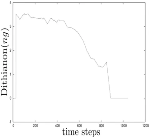
Figure 10. Time evolution at inflow of Dithianon.
Three pesticides applied to apple orchards in the Non Valley and characterized by different physical-chemical properties (Table 1), Pirimicarb, Dithianon, Methoxfenozide, were selected for running the model.
Table 1. Physical-chemical properties of the chemicals selected for model simulations.
Pirimicarb Dithianon Methoxyfenozide
Molecular weight (g/mol) 238.3 296.3 368.5 Melting point (°C) 90.5 225 204.5 Vapor pressure (Pa) 9.70E−04 2.70E−09 1.48E−06 Solubility (g/m3) 3000 0.14 3.3
Log KOW 1.7 3.2 3.7
Half-life in soil (d) 86* 35* 68* Half-life in sediment (d) 195* 0.05* 68** Half-life in water (d) 33.3 0.05* 68**
Chemical half-lives in water (33.3, 0.05 and 68 days, respectively) were used to update concentrations according to decay, as expressed by (16). Hourly chemical loading at the inflow deriving from water runoff in the Novella watershed were calculated for the three chemicals using SoilPlus [11], a dynamic multimedia model based on the fugacity concept developed to investigate the fate organic chemicals in the air/litter/soil system at the local scale. A 10 cm loamy soil compartment divided in 20 sub-layers (thickness: 0.5 cm) and starting from field-capacity conditions was simulated. Precipitation data for the simulation period were acquired from Meteotrentino web-side [18]. Despite realistic applications, rates were used for all chemicals and it was assumed that they were applied directly to the soil layer. It must be remarked that no attempt was made to depict the real agricultural scenario of the Non Valley. For example, only one soil type was used and slope was not considered in runoff calculations. The only intention was to create a realistic environmental scenario for model illustration. Chemical loading at inflow were obtained by multiplying the SoilPlus output values, i.e., hourly amounts of chemical per unit area, by the application area.
Remark 5.1. Reference temperature for vapor pressure is 25°C, while for the solubility is 20°C [24]; for Methoxyfenozide, given the lack of data, half-lives in sediment and water were assumed equal to the one in soil [13]. From these data, it was possible to calculate the hourly average river depth h and the concentrations ci, using the formula:
= $ z| 2h@@3@{ (43)
where niis the number of mole and wiis the atomic mass of
each pollutant, while qt is the total discharge. The time
evolution diagrams of concentrations at inflow (expressed in
ng/L) are reported in figures 9, 10 and 11.
Finally, considering that the concentrations are reduced of 0.5 in 2877120 s, in 4320 s and in 5875200 s for Pirimicarb, Dithianon and Methoxyfenozide respectively, it was possible to find the compounds decaying ratios for ∆t=100s:
rP=0.999975909, rD=0.984082963, rM=0.999988202.
We considered the domain Ω=[0; 3500] partitioned in 875
elements of equal length 4 m. The numbers of nodes were 1751 for the unit width discharge and the pollutants, and 876 for the elevation. The transient studied was 28 hours, that is 104400 s, with ∆t=100 s. For the Schwarz preconditioner we subdivided the domain Ω in 14 sub-domains Ωi (i=1,..., 14),
each one with about 135 nodes, moreover we add the domain Ω0 with 80 nodes. The overlapping consisted of two elements
(4 nodes). Keeping into account that the matrix of (20) is constant in time and that the matrix obtained from its multiplication with the preconditioner is a well-conditioned matrix, this last one was used in all the time steps. On the contrary, the right hand term of (20) changes at every time step so that it had to be multiplied at every step for the pre-conditioner. Consequently, the three preconditioned systems (20) were solved at each step by means of the Schwarz preconditioned iterative Bi-CGSTAB solver in a very efficient way, in fact the number of iterations for each of the three systems was less than 13.
The initial conditions of the flow were obtained simulating a transient so that the depth at inflow was 0.26 m (the same measured at 00:03 on 02/11/2009). The initial conditions of the pollutants were null values.
The boundary conditions were: at inflow Dirichlet for all the variables assigned: in particular for flow the known values h, linearly interpolated every 100 s, and the corresponding values q obtained by the statistical formula (42); for concentrations the known values linearly interpolated every 100 s. At outflow homogeneous Neumann for all the variables.
The source terms of (1)÷(4) were: f=-g(q|q|)/(h7/3K2)
where K=16 and si=0, Si=0. The reaction functions were ai=0 and the physical parameters were: µ=0.001, α=0.003, Γi=0.00001, g=9.81.
For what concerns the results, in figures 12 and 13 are reported, along the domain, the depth and the unit width discharge after 520 time steps, and in figures 14, 15, 16 and 17, 18, 19 are reported the time evolutions of Pirimicarb, Dithianon and Methoxyfenozide at the nodes of abscissa 876 m and 1750 m respectively.
Figure 13. Distribution along the domain of unit width discharge after 520 time steps.
Figure 14. Time evolution at node of abscissa 876 m of Pirimicarb.
Figure 15. Time evolution at node of abscissa 876 m of Dithianon.
Figure 16. Time evolution at node of abscissa 876 m of Methoxyfenoxide.
In figures 20, 21 and 22 are reported the distributions along the domain of the Pirimicarb, of the Dithianon and of the Methoxyfenozide after 520 time steps.
By the graphics can be verified that the computed velocity field is sub-critical everywhere, since the Froude number
Fr=0.23<1, and that the flow is coherent with the boundary conditions imposed. The approximation of the convective term by characteristics allowed a maximum number
CFL=11.25, nevertheless the numerical solution remained stable and accurate. For what concerns the pollutant distributions, by the results can be seen that the most important phenomenon is the convection so that the concentrations are transported along the domain almost constant, see figures 14 ÷ 19.
Moreover, from figure 20, 21 and 22 it can be observed that the compounds are realistically spread out along the river and they are moving with respect of the river current. It can also see, for all the pollutants, the perfect coherence between the concentration value measured at a fixed point x
of the spatial distribution relevant to instant t, and the concentration value measured at a fixed instant t in the time evolution relevant to the point x. The profiles of concentrations are closely related to the physical-chemical properties of the modeled chemicals, mainly log KOW and half-lives, which influences chemical runoff. For example, Pirimicarb shows a rapid decrease in concentration which is due to its extremely high solubility in water and low log KOW; during the first hours of the precipitation event, it is rapidly removed from soil by runoff water. In contrast, both Dithianon and Methoxyfenozide show a slowly decreasing concentration profile; this behavior can be ascribed to higher log KOW and low solubility. Moreover, Methoxyfenozide is characterized by a moderate persistence in the environment (Table 1).
Figure 17. Time evolution at node of abscissa 1750 m of Pirimicarb.
Figure 18. Time evolution at node of abscissa 1750 m of Dithianon.
Figure 19. Time evolution at node of abscissa 1750m of Methoxyfenozide.
Figure 20. Distribution along the domain after 520 time steps of Pirimicarb.
Figure 21. Distribution along the domain after 520 time steps of Dithianon.
5. Conclusions
In this paper a deterministic numerical model for the prevision of the distribution of pollutants in rivers has been presented. The model is based, for the flow, on the 1D Saint Venant equations, i.e. on the hypothesis of constant vertical velocity and hydrostatic pressure, and for the compounds on convection-diffusion and decay equations. The most important numeric features of the model presented are: time advancing by a fractional step scheme that allows for decoupling the physical contributions, and consequently to solve the wave equation with a low computational cost; approximation of the convective terms by means of characteristics so that the computational kernels are reduced to elliptic like ones. The algebraic systems are solved by means of very efficient methods: that relevant to the elevation by a Thomas solver and those relevant to the concentrations by a Schwarz pre-conditioned iterative Bi-CGSTAB solver. Of course, studies relevant to rivers with significant transversal velocity shouldn't be afforded by this model, however for studies on channel flows or on flows of linear segments of rivers it appears to be a promising tool, especially in presence of very long transients. The new model has been tested on three cases which results confirm its accuracy and computational efficiency. The first and second tests have known analytic solutions and the third one is an application to the realistic case of chemical pollution of the Novella River. The expected computational efficiency has been confirmed, in fact the overall Novella transient took 11 minutes of elapsed time on a Toshiba Intel Core I5 Satellite Pro personal computer.
Acknowledgments
The authors thank the Comune di Dambel for having provided the Novella River depth and discharge data, Dr. M. Semplice and the Referees for the helpful comments given.
References
[1] V. I. Agoshkov, D. Ambrosi, V. A. Pennati, A. Quarteroni and F. Saleri, “Mathematical and numerical modeling of shallow water flow”. Computational Mechanics, 11, 280-299, 1996. [2] D. Ambrosi, S. Corti, V. A. Pennati and F. Saleri, “Numerical
simulation of unsteady flow at Po river delta”. Journal of Hydraulic Engineering, 12, 735-743, 1996.
[3] R. Aruba, G. Negro and G. Ostacoli, “Multivariate data analysis applied to the investigation of river pollution”. Fresenoius Journal of Analytical Chemistry, 346, 10-11, 968-975, August 1993.
[4] M. Atallah and A. Hazzad, “A Petrov-Galerkin scheme for modeling 1D channel flow with variating width and topography”. Acta Mechanica, 223, 12, 2012.
[5] J. P. Benquè, J. A. Cunge, J. Feuillet, A. Hauguel and F. M. Holly, “New method for tidal current computation”. Journal of Waterway, Port, Coastal and Ocean Engineering, ASCE, 108, 396-417, 1982.
[6] D. Biasioni, “Analisi delle portate Rio Sass e Torrente Novella”. International report, Comune di Dambel, Trento, Italy, 2009-2010.
[7] S. Bonzini, R. Verro, S. Otto, L. Lazzaro, A. Finizio, G. Zanin and M. Vighi, “Experimental validation of geographical information system based procedure for predicting pesticide exposure in surface water”. Environmental Science Technology, 40, 7561-7569, 2006.
[8] N. Crnjaric-Zic, S. Vukovic and L. Sopta, “Balanced finite volume WENO and central WENO schemes for the shallow water and the open channel flow equations”. Journal of Computational Physics 200, 512-548, 2004.
[9] C. Gold, A. Feurtet-Mazel, M. Coste and A. Boudou, “Impacts of Cd and Zn on the development of Periphytic Diatom communities in artificial streams located along a river pollution gradient”. Archives of Environmental Contamination and Toxicology, 44, 2, 0189-0197, February 2003.
[10] P. Garcia-Navarro and A. Priestly, “A conservative and shape-preserving semi-Lagrangian method for the solution of the shallow water equations”. International Journal for Numerical Methods in Fluids, 18, 273-294, 1994.
[11] D. Ghirardello, M. Morselli, M. Semplice and A. Di Guardo, “A dynamic model of the fate or organic chemicals in a multilayered air/soil system: Development and illustrative application”. Environmental Science Technology, 44, 9010-9017, 2010.
[12] M. E. Hubbard and P. Garcia-Navarro,”Flux Difference Splitting and the Balancing of source terms and flux gradients”. Journal of Computational Physics, 165, 89-125, 2000.
[13] IUPAC FOOTPRINT Pesticides Properties Database, http://sitem.herts.ac.uk/aeru/iupac/ Last accessed: March 26, 2013.
[14] A. C. Kengni Jotsa, “Solution of 2D Navier-Stokes equations by a new FE fractional step method”. PhD thesis, Università degli Studi dell'Insubria sede di Como, March 2012.
[15] A. C. Kengni Jotsa and V. A. Pennati, “A cost effective FE method for 2D Navier-Stokes equations”. Engineering Applications of Computations Fluids Mechanics, Vol. 9, N. 1, 66-83, 2015.
[16] W. Lai and A. A. Khan, “Discontinuous Galerkin method for 1D shallow water flow in non-rectangular and non-prismatic channels”. Journal of Hydraulic Engineering, 138 (3), 285-296, 2012.
[17] J. M. Lescot, P. Bordenave, K. Petit and O. Leccia, “A spatially-distributed cost-effectiveness analysis framework for controlling water pollution”. Environmental Modelling and Software, 41, 107-122, March 2013.
[18] Meteotrentino webside: “http://www.meteotrentino.it/” Last accessed: March 26, 2013.
[19] P. Ortiz, O. C. Zienkiewicz and J. Szmelter, “CBS Finite element modeling of shallow water and transport problems”. ECCOMAS 2004, Jyvaskyla, 24-28, July 2004.
[21] A. Quarteroni and A. Valli, “Domain decomposition methods for partial differential equations”. Oxford Science Publications, 1999.
[22] A. Sharma, M. Naidu and A. Sargoankar, “Development of computer automated decision support system for surface water quality assessment”. Computers and Geosciences, 51, 129-134, February 2013.
[23] L. J. Thibodeaux and D. Mackay, “Handbook of estimation methods for chemical mass transport in the environment”. CRC Press, New York 2011.
[24] C. D. S. Tomlin, “The Pesticide Manual: A World Compendium”. Eleventh ed. British Crop Protection Council, Farhnham, Surrey, UK 1997.
[25] G. Vignoli, V. A. Titarev and E. F. Toro, “ADER schemes for the shallow water equations in channel with irregular bottom elevation”. Journal of Computational Physics, 227, 4, 2463-2480, 2008.
[26] A. Walters, “Numerically induced oscillations in the finite element approximations to the shallow water equations”. International Journal for Numerical Methods in Fluids, 3, 591-604, 1983.