Poverty Changes in Cameroon over the 1996-2007 Period



Samuel Fambon (Correspondence)



sfambon@yahoo.fr



+(237) 69987 4310

This article is published under the terms of the Creative Commons Attribution License 4.0 Author(s) retain the copyright of this article. Publication rights with Alkhaer Publications. Published at: http://www.ijsciences.com/pub/issue/2017-04/

DOI: 10.18483/ijSci.1241; Online ISSN: 2305-3925; Print ISSN: 2410-4477

Poverty Changes in Cameroon over the

1996-2007 Period

Samuel Fambon

1

_

1

Faculty of Economic and Management, University of Yaoundé II – Cameroon

Abstract: This study examines changes in the extent of poverty in Cameroon during the period 1996-2007. More specifically, it investigates the determinants of poverty as well as the contributions of growth and redistribution factors to changes in poverty over a period of 12 years going from 1996 to 2007. The analysis is based on data gathered at the household level by three consecutive household surveys that were conducted in 1996, 2001 and 2007 respectively. The results of the study show that over a period of 12 years, the extent of poverty decreased by more than half in the urban area, while in the rural area, it fell first between 1996 and 2001, and then increased from 50% in 2001 to 55% in 2007. This alarming rate of increase in poverty in the rural area requires a greater attention of the government which should initiate efficient poverty reduction programs. The study also reveals that human and social resources, as well as physical capital, household size, the occupation and the residence region are the main determinants of poverty. Lastly, the decomposition of changes in poverty into growth and redistribution components indicates that during the sub-period 1996-2001, growth and redistribution contributed to the reduction of urban poverty, whereas redistribution almost did not have any impact on the reduction of rural poverty. On the other hand, over the sub-period 2001-2007, the reduction of poverty in the urban area is mainly explained by the effects of growth and redistribution, while in the rural area, the increase in poverty is essentially explained by the unfavourable growth effect. The implications of the results of the study for a pro-poor policy are discussed.

Keywords: Poverty, determinants, growth, redistribution, Cameroon

1. Introduction

In reaction to a severe economic crisis1 characterized by a negative economic growth rate of -2.3% over the period 1987-19942, Cameroonian authorities were forced towards the end of the 1980s and at the beginning of the following decade, to adopt and apply the principles of a healthy management of the economy by implementing a series of economic recovery policy measures, which mainly included stabilization and economic reforms, as well as structural adjustment programs aiming at the liberalization of the economy, to which were added the practice of good governance as one of the main conditionalities for receiving international financial assistance. The application of these programs, combined with the devaluation of the CFA Franc relative to the French Franc which took place in January 1994, resulted in economic recovery and an acceleration of the economic growth rate of about 4.5% per year over the period 1995-2000, and then in

1

For a description of the economic crisis in Cameroon, see for instance Aerts et alii (2000).

2

See Charlier and N’Cho-Oguie (2009).

a slowing down of the real GDP growth rate to a 3.4% yearly average over the period 2000-20073.

However, to our knowledge there exists no serious study4 which deals with changes in the extent of

3

Fambon et alii. (2014).

4

http://www.ijSciences.com

Volume 6

– April

2017 (04

)

49

poverty in Cameroon over the period 1996-2007, and which simultaneously uses the three consistent and comparable databases of the household surveys that the country possesses. And yet, the implementation of stabilization policies and structural reforms, as well as the devaluation of the national currency in any country, may have a major impact on poverty and inequality.

The present study fills this gap by investigating temporal changes in poverty in the rural and urban areas over a period of twelve years going from 1996 to 2007. In particular, we analyze not only the relative contributions of growth and redistribution factors in changes in poverty during the period, but also a few determinants of poverty by using household level data derived from three Cameroonian household surveys namely, ECAM1, ECAM2 and ECAM3 conducted by the National Institute of Statistics (NIS) of Cameroon respectively in 1996, 2001 and 2007. The analysis of these data makes it possible to widen the debate on the interrelations between economic growth and the dynamics of poverty by providing new evidence at the microeconomic level from a Sub-Saharan African economy such as Cameroon’s. In addition, decision-makers also need better information on the evolution and causes of poverty because in recent years, the government had very few resources at its disposal to finance poverty reduction programs. Thus, a better understanding of changes in poverty and its determinants in Cameroon may facilitate both an effective conception of social policies, and greater efficiency in the poverty reduction programs.

This study is structured around 8 sections. After the introduction in Section 1, Section 2 presents the data and the methodology of the study. Section 3 examines temporal changes in poverty levels in Cameroon as a whole, while Section 4 deals with these changes in the rural and urban areas of the country. This section is followed by Section 5 which is devoted to the stochastic dominance test, and which helps us see the robustness of our poverty comparisons in the choice of alternative poverty lines. Section 6 analyzes the determinants of rural and urban poverty, and Section 7 breaks down the temporal change in poverty into components associated with growth and redistribution factors. Lastly, Section 8 concludes the study and proposes some policy implications for the reduction of poverty.

2.Methodology and Data 2.1 Methodology

2.1.1The indicator of welfare

In the context of this study, the monetary value of household consumption expenditure is chosen as a measure of welfare for the analysis of poverty. Consumption is a preferred welfare measure in developing countries for a number of reasons (Deaton (1997)). Firstly, consumption is a better welfare indicator for a person because it is closely linked to welfare than income. Secondly, from an empirical point of view, it can be shown that consumption expenditures are measured with greater precision than incomes, above all in the case where a large share of these incomes comes from the informal sector of the economy. This argument is particularly pertinent in a developing country like Cameroon where, as in the case of the ECAM1 survey which is one of the databases used in this study, 8.6 % of the households declared an income that was higher than expenditures! In other words, incomes were largely underestimated everywhere, a situation which excludes the use of income as a household welfare indicator in the present study. Finally, consumption is less volatile than income, and it may be a better indicator of the actual living standard of a household.

In addition, in this analysis we will take account of the differences in the size and composition of different households, and as a consequence, we will use household expenditure per adult equivalent as a welfare measure (Deaton and Muellbauer (1980))5. The indicator of living standards retained in the context of the analysis of the evolution of poverty over the period 1996-2001 comprises: food and non food expenditures (clothing and footwear, household equipments, transports and communications, various services and housing services), the use value of

5

*Household aggregate consumption comprises food expenditures (including meals taken outside the household), non monetary food consumption resulting from home consumption, and donations; the purchase value of non durable goods and services; an estimate of the use value of durable goods, and the imputed value of housing for those households who own their accommodations or are housed for free by a third party.

http://www.ijSciences.com

Volume 6

– April

2017 (04

)

50

durable goods common to both surveys, and auto consumption and transfers in kind received. Once evaluated according to the same approach, the expenditures of 1996 and of 2001 are corrected of the temporal and spatial fluctuations in prices, with the year 2001 taken as a reference year. This double deflation of aggregate consumption makes the 1996 expenditures and those of 2001 directly comparable in order for the stochastic dominance tests to be conducted (see NIS (2002), and Fambon and Tamba (2010) for more details)).

To undertake inter-temporal acceptable comparisons of poverty, we have deflated the household consumption expenditures per adult equivalent of 2007 to bring them back to the level of those of 2001. To do this, the household consumption expenditures per adult equivalent of 2007 are divided by a deflator, that is to say, the ratio of the poverty line of 2007 by that of 20016.

2.1.2 The Poverty Line

In general, poverty lines are cut-off points; households with incomes or consumptions under this value are considered as being poor. An absolute poverty line (that of 2001), is used in the present study to estimate the incidence of poverty, and the indices of the depth and severity of poverty in Cameroon. This poverty line was calculated by the NIS using the basic needs costs method, and it comprises the food poverty line and the non-food poverty line.

The food poverty threshold is calculated from the consumption costs of a certain number of kilo-calories which makes it possible to subsist. The norms used to calculate these consumption costs vary from 1800 to 3000 kilo-calories per adult and per day. In 2001, the NIS adopted the use of 2900 kilocalories per adult-equivalent per day. A basket of the 61 goods most consumed by households which represent nearly 80% of food consumption was chosen. The rise in value of this basket at the price of Yaoundé, the capital city of Cameroon, has made it possible to determine the food poverty threshold

z

a.

For the non food threshold, this norm does not exist. The NIS has taken as a food threshold, the non-food consumption of households whose total consumption per adult-equivalent is just equal to the poverty threshold (Ravallion (1996)). In the case of

6

The poverty lines of 2007 and 2001 are respectively CFAF 269 443 per adult equivalent per year and CFAF 185 490 per adult equivalent per year; this deflator is given by the following ratio: 269443/185490=1.4526.

Cameroon, the non food threshold was estimated indirectly using linear regression. The dependent variable of this model is the share of household food expenditures, and its independent variables are the logarithm of the ratio of total household expenditures over the food poverty threshold, and other household consumption variables. The ordinate at the origin of this regression (a) is the share of household food expenditures whose total expenditure is equal to the poverty threshold, while (1-a) (in the equation 1 below) is their non-food share. Consequently, the total poverty threshold is:



1







a a a

z



z



z



a



z

z



a

(1)

The NIS reports on the dimensions of poverty in Cameroon indicate that the total poverty line in 2001 was equal to CFAF 185490 in total annual expenditure per adult-equivalent; that of 2007 was equal to CFAF 269443 in total annual expenditure per adult equivalent. For more details concerning the calculations of these poverty thresholds, see INS (2002), INS (2008), and Fambon et alii (2014).

2.1.3 The Measure of Poverty

Once the welfare indicator is chosen and the poverty line estimated, the poverty measure to be used must be chosen. Three different poverty measures are used in this study, and they are the poverty ratio, the index of the depth of poverty, and the index of the severity of poverty. All of these measures are members of the additive and decomposable class of poverty measures proposed by Foster, Greer and Thorbecke (1984)7, and their general formula is given by:

 

1

1

q i

i

Z

y

P

FGT

n

Z

 















_

_







(2) where,

n

is the size of the population (i.e. the number of individuals or households in the population);

q

represents the number of poor persons (it is the index of the individual whose expenditure is

7

Foster-Greer and Thorbeck (1984) and others have

http://www.ijSciences.com

Volume 6

– April

2017 (04

)

51

exactly situated on the poverty line);

z

is the poverty line;

y

_i is the level of expenditure per adult equivalent of household

i

( it is assumed that individuals are ordered by increasing order of expenditure), and



is the weighting parameter of poverty (





0

).

When  = 0, the

FGT

index becomes

P

0



q n

(i.e. the poverty ratio) which measures the incidence of poverty, that is, the number of poor persons expressed as a percentage of the total population. It is the most frequently used poverty measure. The main advantage of this statistic is that it is simple as its formula indicates.

On the other hand, When  = 1, we obtain the poverty index

P

₁ (the index of the depth of poverty) which is the product of the poverty ratio

P

₀

multiplied the average expenditure gap among the

poor

G



, which means that

P

₁

P G

₀





with

1

q

i i

G

G

q









8

(3).

The index

P

₁ therefore takes into consideration both the incidence of poverty and the average depth of poverty. Therefore, this is about an index which measures the depth of poverty. This index is only sensitive to the situation of the average poor and does not take into consideration the poorest persons among the poor.

If  = 2, we obtain the index

P

₂ which measures the severity of poverty, and it is expressed as

follows:

2

2

1

1

1

q

i

i

y

P

n



Z







_



_







(4)

This

P

2 index is sensitive not only to the incidence

and to the depth of poverty, but also to the distribution of resources among the poor. A stronger inequality among the poor implies a higher value of

2

P

. The index of the severity of poverty has the main advantage of comparing the policies that aim to reach the poorest of the poor, but it is more difficult to interpret and is less intuitive than the preceding two poverty measures.

8

The expenditure gap of household

i

may be defined as the percentage of the deficit of the expenditure level that lies under the poverty threshold, which is to

say that

G

_i



z

y

i



z





.

Rather than being alternative poverty measures, the preceding three poverty measures provide complementary insights into the standard of living of the population.

2.2 The Data

The analysis of poverty in this study is based on data at the household level, and they were gathered by the three Cameroonian household surveys ECAM1, ECAM2 and ECAM3 which were conducted respectively in 1996, 2001 and 2007 by the National Institute of Statistics (NIS) of Cameroon. The objective of these household surveys was to collect reliable data on changes in the living standards of Cameroonian households, and each of the above surveys had its own objective. The objective of ECAM1 was to measure the impacts of the economic crisis and of the structural adjustment policies on the living conditions of households, and to analyze the interrelations between the living standards. The ECAM2 survey was concerned with the measurement of the living conditions of households in Cameroon in 2001. This survey mainly aimed at putting in place the bases of a permanent monitoring and evaluation system of the living conditions of households in general, and of the poverty reduction program, in particular, thus making it possible to establish a situation of reference which will serve periodically to appreciate the impacts of programs and policies implemented in Cameroon. As to the ECAM3 survey, it aimed to update the poverty profile of the year 2001, to appreciate the progress realized as far as poverty reduction is concerned, to achieve the objectives of the millennium development goals (MDGs) and to feed the revision of the Poverty Reduction Strategy Paper (PRSP) adopted by the Cameroonian government in April 2003.

The sample sizes of the ECAM1, ECAM2 and ECAM3 surveys respectively amount to 1731, 10992 and 11369. These surveys are representative at the national level, and the contents of their questionnaires are conceived to permit data collection not only on the individual characteristics of households, but also on the consumption of household incomes. These surveys are highly comparable in terms of the sampling procedure and the data gathering methodology. For more details on the ECAM1, ECAM2 and ECAM3 surveys see for instance, NIS (1996), NIS (2002), NIS (2008), Fambon and Tamba (2013) and Fambon et al. (2014).

http://www.ijSciences.com

Volume 6

– April

2017 (04

)

52

Table 3.1 below provides an overall view of the evolution of poverty in Cameroon and according the

residence area of the household head during the period 1996 - 2007.

Tableau 3.1: Trends in Monetary Poverty over the Period 1996- 2007

Cameroon Urban Rural

1996 2001 2007 1996 2001 2007 1996 2001 2007

0

P

0.5327 (0.0326) 0.4022 (0.0146) 0.3988 (0.0134) 0.4137 (0.0297) 0.2211 (0.0115) 0.1217 (0.0085) 0.5964 (0.0464) 0.4988 (0.0193) 0.5502 (0.0176) 1

P

0.1908 (0.0167) 0.1414 0.0085) 0.1231 (0.0062) 0.1466 (0.0134) 0.0631 (0.0039) 0.0281 (0.0024) 0.2145 (0.0242) 0.1832 (0.0122) 0.1750 (0.0086) 2

P

0.0900 (0.0095) 0.0698 (0.0061) 0.0503 (0.0031) 0.0691 (0.0074) 0.0266 (0.0020) 0.0096 (0.0010) 0.1012 (0.0138) 0.0928 (0.0090) 0.0724 (0.0045)

Note: Figures in parentheses represent standard errors

Source: Computed by the Author from ECAM1, ECAM2 and ECAM3 Survey data

At the national level, we observe the fact that monetary poverty decreased over the period 1996 - 2001, and remained almost stable between 2001 and 2007. Actually, between 1996 and 2001, all the poverty measures, namely

P

₀,

P

₁, and

P

₂, indicate a non negligible reduction of this phenomenon. The percentage of individuals in the Cameroonian population who were living in poverty in 1996 (that is about 53%) decreased considerably five years later to approximately 40% in 2001. This reduction in poverty at the national level did not only concern the fall in the number of poor individuals, but also the decrease in the indicators for measuring the depth and severity of poverty, which assign a greater weight to the poorest of the poor. Actually, the index of the depth of poverty has witnessed a reduction of 5 percentage points during the period, going from 19% in 1996 to 14% in 2001, and the index of the severity of poverty (

P

₂) also decreased by two percentage points over the period.

On the other hand, we note the near-stability of poverty over the period 2001-2007, characterized by a marginal decrease in the incidence, the depth and the severity of poverty. Actually, the poverty ratio went from 40.2% in 2001 to only 39.9% in 2007. This result shows that Cameroon did not take advantage the macroeconomic stability and of the opportunities offered during this period, notably the resources engaged following the attainment and completion of the decision point of the Highly Indebted Poor Countries (HIPC) Initiative.

The depth of poverty also remained stable over the period, going from 12.8% in 2001 to 12.3% in 2007. In other words, individuals who remained poor in 2007 did not witness a substantial fall in their consumption deficit relative to the year 2001. This result thus shows that the poor did not take advantage of the effects of economic growth during the period,

in order for the average gap between their consumption level and the poverty threshold to witness a significant reduction. Finally, as to the index of the severity of poverty, it went from 5.55% in 2001 to only 5.03% in 2007.

4. Trends in Poverty According Residence Area

Although Cameroon, as compared with other countries of Sub-Saharan Africa is a relatively urbanized society, more than 65% of its population lives in the rural area. It is therefore useful to also analyze poverty according to rural and urban areas. Table 3.1 above shows the incidence, depth and severity of poverty for each year of the study and separately for the urban and rural areas.

As may be observed from this table 3.1 above, the level of poverty in the rural area was more severe in the rural area than in the urban area in 1996, 2001 and 2007. For instance, in 1996, about 60% of the rural population lives in poverty. The corresponding figure for the urban area is 41%. The estimates of the index of the depth of poverty and that of the severity of poverty are even less than half of those of its rural counterpart. Both areas have witnessed a decrease in poverty between 1996 and 2001.

In fact, between 1996 and 2001, poverty decreased by more than 19 percentage points in the urban area, thus falling almost by half from 41% to 22% during the period. This was not restricted exclusively to the poverty ratio, it also affected all the FGT poverty indexes, particularly the depth and severity of poverty (

P

1 and

P

2) which witnessed non negligible falls of

http://www.ijSciences.com

Volume 6

– April

2017 (04

)

53

worsened (See Fambon et al., 2005). However, in spite of this very considerable improvement, almost 22% of the urban population was still living under the poverty threshold 2001.

In the urban area, one observes a decrease in the poverty rate of 5.7 percentage points between 2001 and 2007, contrary to the rural area which rather witnessed an increase of 3 percentage points in the incidence of poverty over the period.

However, the indicators of the measure of the depth and the severity of poverty, which assign a greater weight to the poorest of the poor, witnessed a less favourable evolution in the urban area over the same period, with clearly a less significant registered by the indicator of the depth of poverty (

P

₁) and the index of the severity of poverty (

P

₂) relative to the measure

P

₀ of poverty. In the rural area, on the other hand, one observes a slight increase in the depth of poverty (

P

₁) and a weak decrease in the severity of poverty (

P

₂)relative to the poverty ratio

P

₀.

Now we are going to check the robustness of the preceding results with the help of the stochastic dominance technique.

5. Stochastic Dominance Tests

When one compares poverty measures over time or between groups, it is important to test the robustness of the changes observed in the poverty indexes. In fact, the changes observed could depend on the poverty line selected and at their most extreme, the use of two different poverty lines may suggest changes in opposite directions. To compare poverty measures by using stochastic dominance techniques may help to establish the robustness of the ordinal classifications of poverty.

Stochastic dominance of the first order implies the comparison of cumulative distribution functions of the indicator of welfare (income or consumption for each of the years of the survey, or for the different household groups for which poverty comparisons are made. Thus, by putting the income of the household per adult equivalent on the horizontal axis, and the cumulative percentage of the population at the successive levels of household income per adult equivalent on the vertical axis, we can plot the poverty incidence curve (PIC) or cumulative distribution curve of the household per adult equivalent. It this curve, for let’s say year 1, lies entirely at the right and under that of year 2, then we can infer that that poverty has increased without ambiguity between year 1 and year 2 without taking account of either the place where the poverty line is

plotted, or of the poverty measure used (at least as far as the poverty measure has certain desirable properties).

If it is found that first order dominance is confirmed between two different years or between two different groups9, this implies that all the FGT poverty measures including the poverty ratio, the index of the depth of poverty and the index of the severity of poverty in the first year or group is higher in the first year or group for all the poverty lines. .

If two incidence curves cross, then certain poverty lines or poverty measures are likely to be classified differently. In this situation, certain restrictions on the structure of the poverty measure most be imposed. If we have to limit ourselves to the decomposable poverty measures

P

₁ and

P

₂ which respectively reflect the depth and severity of poverty, then the conditions of second order and third order dominance may be applied to classify the levels of poverty. The condition of second order dominance stipulates that if the area under the curve of the deficit of poverty (given by the area under the cumulative distribution) for year 1 is lower than that of year 2, then there is an unequivocal increase in poverty from year 1 to year 2. If this test is not conclusive (i.e. if the two curves cross), then we can apply the dominance test of third order which requires that, for an unambiguous comparison of poverty for all the poverty lines, the curve of the deficit of poverty is everywhere higher in one of the two to be compared. For more details on the discussion on dominance tests, see Ravallion (1994), and Davidson and Duclos (2000).

The robustness of the preceding results is evaluated with the help of the stochastic10 dominance technique which requires the curves of the expenditure distribution to be plotted for the different residence areas or the years to be compared.

Figures 3.1 and 3.2respectively compare the poverty incidence curves of Cameroon over the periods

9

Consequently, stochastic dominance was a theoretical movement outside cardinal poverty, and towards an emphasis on research for the consistence and robustness in the evaluation of poverty. If first order stochastic dominance is demonstrated, then second order and third order stochastic dominances are guaranteed.

10

http://www.ijSciences.com

Volume 6

– April

2017 (04

)

54

2001 and 2001-2007. It emerges from Figure 3.1 that from a level of approximately 90.000 CFAF per adult equivalent per year, the distribution of the expenditures of 2001 dominates that of the year 1996. In other words, for any poverty line considered from this minimum level, poverty is less pronounced in 2001 than in 1996.

Figure 3.2 presents the first order stochastic dominance test which corroborates the preceding conclusion on poverty in Cameroon during the period

2001-2007. In other words, for a large range of poverty lines, and with no hypotheses on the poverty threshold, it seems that poverty decreased unequivocally for a large range of poverty lines, between 2001 and 2007. The poverty incidence curves validate the conclusion that poverty decreased without any methodological hypothesis. In fact, when first order stochastic dominance is confirmed, not only the comparisons of poverty are robust across the poverty lines, but they are robust cross a wide range of poverty measures (Atkinson (1987)).

Figure 3.1: Poverty incidence curve for Cameroon, 1996–2001

Figure 3.2: Poverty incidence curves for Cameroon, 2001–07

Source: Computed by the author from ECAM1, ECAM2 and ECAM3 data.

http://www.ijSciences.com

Volume 6

– April

2017 (04

)

55

the other hand, this result is only valid from a poverty threshold of about 90.000 CFAF per adult equivalent per year. In general, poverty declined between 1996 and 2001, but this reduction was more significant in the urban area than in the rural area for any poverty index considered.

http://www.ijSciences.com

Volume 6

– April

2017 (04

)

56

6. The Determinants of Poverty: A Multivariate

Analysis

To elaborate a poverty reduction strategy, it matters to clarify its determinants as well as the factors likely to affect this strategy. In the present section, we model the determinants of poverty levels by taking the logarithm of real household consumption expenditures per adult equivalent divided by the poverty line (welfare ratio), which we regress on a certain number of explanatory variables characteristic of the household and the community in which households reside11. The dependent variable is the

11

Numerous authors such as Glewwe (1991), Mukherjee et al. (2003), Canagarajah and Pörtner (2003), Banque Mondiale (2003), and Audet et al. (2006) propose many theoretical arguments in favour of the continuous approach to the detriment of the discrete approach as far as the modelling of poverty determinants is concerned.

logarithm of the « welfare ratio » which is a proxy for the standard of living. The welfare ratio is defined as consumption expenditures per adult equivalent deflated or divided by a national poverty line12. This indicator reflects living standards as a multiple of the poverty line. A unitary value for the welfare ratio means that the household has its level of consumption expenditure per adult equivalent exactly at the level of the poverty line. A higher welfare ratio value means higher living standards.

12

http://www.ijSciences.com

Volume 6

– April

2017 (04

)

57

In this paper, the independent or exogenous variables used include: (1) Sex of the household head (Male or Female); (3) Regions in which households reside (divided into 12 regions: Douala, Yaoundé, Adamaoua, Centre, East, Far-North, Coast T, North, North-West, West, South, and South-West); (4) Educational levels of the household head (categorized into 5 levels: 1. without level, 2. primary, 3. Secondary first cycle, 4. Secondary second cycle, 5. Higher Education); (5) Occupation of household head (categorized in 4 kinds of jobs, including executive, qualified employee, unskilled worker and manager); (6) branches in which the household head works (categorized in four sectors, namely: the agricultural sector, the industrial sector, the trade sector and the services sector.): (7) household composition variables (household size); (8) the age group of the household head (categorized in three household-head age groups, namely the 30-39 age group, the 50-59 age group, and the 60 or more age group); (9) matrimonial status of household head (married); (10) the area of cultivated land and equity capital; (11) access to infrastructures measured by the time spent to reach those infrastructures (the time spent to reach a food market, the time spent to reach an asphalted road); (12) the other variables introduced in the model are: «a household member is a member of an association»; «the household head obtained a business credit».

Several of the variables mentioned above are category-specific (i.e. dummy variables). Consequently, in running our regressions it is necessary to leave one category of variables as a group of reference. Such categories are: Yaoundé, male household head, the household head has no spouse, the household head has no education, one household member is not a member of an association, the household head has not obtained a credit, etc.

It is reasonable to expect the coefficients of the expenditures predicted for the rural area to be different from those predicted for the urban area13.

13

Most poverty studies in developing countries have divided their samples into at least two categories. To a minimum, the households analyzed are divided into those of the urban area and those of the rural area. This division is chosen because the factors affecting poverty are likely to be significantly different in the urban area as compared with the rural area.

Moreover, a household is considered as being urban if it resides in an area with population of more than 50000 inhabitants; if the number of inhabitants is lower than that, the household is considered as rural. These definitions of rural and urban residency are the

This implies that separate analyses should be carried out for the rural and urban samples. The results derived from the regression analyses of the rural and urban areas for year 2007 are presented in Table 214.

The results are almost standard for this type of model. The coefficient of determination (R2) is 43 percent for the regression in the urban area and 38 percent for the regression in the rural area. The explanatory powers of the rural and urban models are comparables to those of similar studies on the determinant of poverty, notably in Egypt (Datt and Jolliffe, 1999) and in Mozambique (Datt, et al., 2000). As a consequence, the results of this study may be considered as being reasonable, for their coefficients of determination turn approximately around the R2s found in the studies mentioned above.

.

Since the dependent variable is in the form of a logarithm, the coefficient estimates of the regressions measure the percentage changes in the welfare ratio induced by unit changes in the independent variables.

standard definitions used by the Cameroon National Institute of Statistics (NIS).

14

http://www.ijSciences.com

Volume 6

– April

2017 (04

)

58

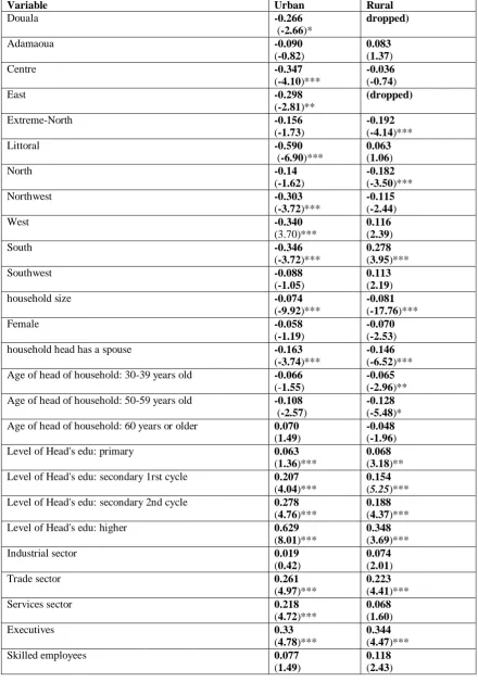
Table 2: Determinants of Urban and Rural Consumption Expenditure, 2007

Variable Urban Rural

Douala -0.266

(-2.66)*

dropped)

Adamaoua -0.090

(-0.82)

0.083

(1.37)

Centre -0.347

(-4.10)***

-0.036

(-0.74)

East -0.298

(-2.81)**

(dropped)

Extreme-North -0.156

(-1.73)

-0.192

(-4.14)***

Littoral -0.590

(-6.90)***

0.063

(1.06)

North -0.14

(-1.62)

-0.182

(-3.50)***

Northwest -0.303

(-3.72)***

-0.115

(-2.44)

West -0.340

(3.70)***

0.116

(2.39)

South -0.346

(-3.72)***

0.278

(3.95)***

Southwest -0.088

(-1.05)

0.113

(2.19)

household size -0.074

(-9.92)***

-0.081

(-17.76)***

Female -0.058

(-1.19)

-0.070

(-2.53) household head has a spouse -0.163

(-3.74)***

-0.146

(-6.52)*** Age of head of household: 30-39 years old -0.066

(-1.55)

-0.065

(-2.96)** Age of head of household: 50-59 years old -0.108

(-2.57)

-0.128

(-5.48)* Age of head of household: 60 years or older 0.070

(1.49)

-0.048

(-1.96) Level of Head's edu: primary 0.063

(1.36)***

0.068

(3.18)** Level of Head's edu: secondary 1rst cycle 0.207

(4.04)***

0.154

(5.25)*** Level of Head's edu: secondary 2nd cycle 0.278

(4.76)***

0.188

(4.37)*** Level of Head's edu: higher 0.629

(8.01)***

0.348

(3.69)***

Industrial sector 0.019

(0.42)

0.074

(2.01)

Trade sector 0.261

(4.97)***

0.223

(4.41)***

Services sector 0.218

(4.72)***

0.068

(1.60)

Executives 0.33

(4.78)***

0.344

(4.47)***

Skilled employees 0.077

(1.49)

0.118

http://www.ijSciences.com

Volume 6

– April

2017 (04

)

59

Unskilled workers -0.089

(-1.49)

-0.029

(-0.56)

Managers (bosses) 0.244

(2.64)*

0.182

(3.84)*** Head is a member of an association 0.075

(2.34)

3.04

(3.04)** Travel time to market place -0.057

( -2.05)**

-0.024

(-2.74)* Travel time to reach an asphalted road -0.027

(-1.90)

-0.019

(-2.89 )** Area of land cultivated 0.048

(3.18)**

0.065

(4.59)*** Head obtained a credit 0.201

(3.09)**

0.173

(3.56)***

Intercept 13.287

(123.30)***

12.827

(212.46)***

R2 = 0.43 R2 = 0.38

F-statistic (33, 1147) = 21.77

F-statistic (31, 3004)=

47.91

Prob. > F = 0.000 Prob. > F = 0.000

1181 3036

Notes: - Dependant variable is log of welfare ratio.

- Robust t- statistics are between parentheses.

- *** Significant at the 1% level; ** significant at the 5% level; * significant at the 10% level.

- Regressions with robust standard errors.

Source: Calculations of the author using the data of the Cameroonian household survey Ecam3

Household demographic characteristics are closely associated with consumption expenditures per adult equivalent.

The evidence derived from cross-section data suggests that large-sized households are likely to be poor. Such is also the case in Cameroon as shown by the regression results presented in Table 2 above. In effect, household size is significant and negatively associated with consumption expenditures per adult equivalent both in the rural and urban areas. This result implies that large-sized families usually have lower expenditures per adult equivalent, a situation that is likely to increase the probability of poverty.

Regression results show that in urban areas, households whose heads are women have, ceteris paribus, a consumption level which is 6 percent lower than that of households headed by men. In the rural area, this percentage is 7 percent. Thus, contrary to the results derived from the descriptive analysis of the preceding section, households headed by women tend to be more vulnerable when they are compared with those headed by men with similar characteristics. The fact that households headed by women have a lower poverty level may therefore be due to other factors such as the composition of the

household which is more favourable to households headed by women15.

Household heads’ age groups exert some significant and negative influences on consumption expenditures, and hence on poverty both in the rural and urban areas.

The results stemming from the rural and urban regression equations indicate that education is an important determinant of expenditures per adult equivalent. The coefficients of most of the education variables are statistically significant and quite large in the urban and rural areas alike. In the urban area, having a primary level of education increases expenditures by about 6.3% relative to those of uneducated persons; this comes from the coefficient

15

http://www.ijSciences.com

Volume 6

– April

2017 (04

)

60

0.063, and from the fact that the dependent variable is in the form of a logarithm. This effect amounts respectively to 20.7%, 27.8%, and 62.9% for households whose heads have a 1st cycle secondary, 2nd cycle secondary, and higher levels of education16.

The institutional sector where the individual exerts his activity and the branch in which he works are also correlated with poverty. The estimation results of the regression model show that there is a premium for a household whose head is a manager, a qualified employee or a director. In the urban area, and respectively in the rural area, a household whose head is a manager has a level of consumption per adult equivalent which is 33% (respectively 34.4% in the rural area) higher than that of a household whose head is self-employed, a mother’s help or an apprentice. For a household whose head is a director, this gain amounts to 24% in the city and 18% in the countryside.

In addition, regarding the activity branch of the household head, the estimation results of the regression model also show that there is a premium (gain) for households whose heads work in industry, trade, and services as compared with households whose heads work in agriculture.

Actually, the fact of working in the trade sector in the urban area induces an increase in consumption per adult equivalent of 26% relative to a household whose head works in agriculture; in the rural area this percentage amounts to 22.3%. Similarly, the fact of working in the services sector in the urban area leads to an increase in consumption per adult equivalent of 22% relative to a household whose head works in agriculture; this percentage is equal to 7% in the rural area. The estimation results of the model confirm the fact that there is a fall in consumption if the household head works in agriculture, thus testifying to the vulnerability of the household concerned.

Access to credit by a household head who plans to engage in agriculture or business also plays an important role in the determination of household living standards. In effect, we note that access to credit by the household head positively and significantly affects living standards both in the urban

16

Strictly speaking, to have a primary level of education in the urban area increases expenditures by about 7% (i.e., exp (0.063)-1) relative to uneducated persons. Similarly, this effect amounts respectively to 23%, 32% and 88% for households whose heads have secondary education first cycle, secondary education second cycle, and higher education.

and rural areas. In the rural area, the coefficient associated with the variable « access to credit » is significant at the 1% significance level17. In addition, the average welfare level of households that have obtained a credit in the rural area is 17.4% higher than that of households that did not have access to credit. This result is similar to that of the study by Geda et al. (2006) on Ethiopia according to which credit is an important component in smoothing out household consumption and, as a consequence, it is pro poor because it increases household welfare.

Production assets and issued capital are positively associated with household consumption and welfare. In effect, the ownership of land increases the level of household consumption per adult equivalent; however, the impact of this variable is weak, and this tends to suggest that other elements such as the means of production should be associated to land.

In addition, membership in any association improves the level of consumption per adult equivalent by 6% and 7.5% respectively in the rural and urban areas. Actually, associations play an important role in improving access to credit when it comes to financing income-generating activities, among others. Moreover, associations more often play the role of insurance (companies) for their members in case of illness, death, etc. However, it should be noted that there exists a double causality, since the level of consumption can incite a household to belong to an association.

The regressions also highlight the impact of access to infrastructures on the welfare ratio. The results derived from regression analysis suggest that the absence of infrastructures contribute to the exclusion of some households from the market, and from income-generating opportunities. The coefficient estimates of the average time span spent to reach an asphalted road or a food market are significant in the rural area. The negative signs of the coefficients show the absence of infrastructures and the enclosure of rural areas; a situation which may induce high transaction costs that are likely to reduce the welfare of populations.

Finally, regression results also show differences between the regions of the country. In the urban area and compared with Yaoundé which is the region of reference for our model, all the other regions of the

17

http://www.ijSciences.com

Volume 6

– April

2017 (04

)

61

country are disadvantaged relative to Yaoundé. Concerning the rural area, all the regions (save for the Extreme-North, the North, and the Northwest) have an advantage relative to Yaoundé.

7. Decomposition of the Reduction of Poverty

In the preceding section, we have seen poverty changes over time. One question remains without an answer: how many poor people benefited from the economic growth that occurred during the period 1996-2007 and during the sub-periods 1996-2001 and 2001-2007? To answer this question, we decompose poverty reduction into two components, one due to

growth and the other to redistribution (i.e. changes in income distribution). Following the method of Datt and Ravallion (1992), we denote the poverty index

,

_t

t

z

P

L















_{as a function of average income and of} the distribution of income at time

t

, where



is the average income given the poverty line

z

, while

L

is the Lorenz curve or the distribution of income/expenditure at time

t

. The decomposition equation may be written as follows:

2 1 1 1 2 2

2 1 2 1 1 1

,

,

,

,

,

,

z

z

z

z

z

z

P

L

P

L

P

L

P

L

P

L

P

L

R















 































_



_{ }





_













































 











₍₅₎

The left hand side of this equation is poverty reduction between periods 2 and 1. In the second member of this equation, the first part is the growth

component by assuming that the distribution

L

1 _has

remained constant. In other words, the growth component is the change in poverty which could have occurred if growth in average expenditure had taken place without any change in the initial expenditure distribution.

The second part of this equation is the redistribution

component when average consumption



1 _is

constant. In other words, the redistribution (or inequality) component is the change which could have occurred if the expenditure distribution had changed from its initial distribution to its final distribution without any change in the average expenditure; and R is the residual which is equal to the difference between growth components measured relative to the final and initial expenditure distributions. By the same token, the residual is equal to the difference between the components of inequality measured relative to the final and initial average expenditures.

If the growth component is the biggest part of the change in poverty, then this indicates that growth has played a more significant role than distribution in realizing changes in poverty, and vice-versa.

Tables 3 and 4 show the decompositions of poverty using the incidence of poverty to analyze the changes in poverty between 1996 and 2001, and between 2001 and 2007 in Cameroon taken as a whole, and in the rural and urban areas of the country.

The examination of figures in Table 3 shows that growth played a dominant role in the reduction of the incidence of poverty at the national level between 1996 and 2001, while the redistribution component18 of poverty reduction was less strong. In fact, growth on the whole played a predominant role in the reduction of poverty, for 11.8 percentage points in the reduction of the incidence of poverty during this sub-period of time are attributable to growth. The redistribution component only explains 1.80 percentage points in the reduction of poverty at the national level, while the interaction term increases the incidence of poverty by about 0.6 percentage points. This result is not surprising because this time period represents a period of high growth with an annual increase of about 4.8% in real GDP19.

The drivers of poverty reduction in the rural and urban areas over the sub-period 1996-2001 may be summarized as follows:

In the rural area, growth was stronger and the 11.35 percentage points of rural poverty reduction are essentially attributable to the growth effect. The redistribution effect only explains about 1% of the reduction in the incidence of rural poverty.

18_{It is important to note that “redistribution” is used}

here as a term that defines changes in the Lorenz curve and inequality, instead of any specific program which targets the poor and redistributes wealth. The redistribution component may be positive even in the absence of such a program, as long as the consumption of the poorest percentiles increases faster than the consumption of the richest portions of the population.

19

http://www.ijSciences.com

Volume 6

– April

2017 (04

)

62

In the urban area, both growth an redistribution explain the reduction of poverty, with 11.03 percentage points of urban poverty reduction being

attributable to growth, while only 6.3 percentage points of poverty reduction are attributable the redistribution of consumption.

Table 3: Changes in the incidence of poverty between 1996 and 2001 decomposed into growth and redistribution effects according to residence area.

Areas Growth component Redistribution

component

Residual Total change in

poverty

Urban -0.1103 -0.0630 -0.0195 -0.1928

Rural -0.1135 -0.0106 0.0264 -0.0974

Cameroon -0,1180 -0,0180 0, 006 -0,1310

Source: Computed by the author from ECAM1 and ECAM2 survey data.

The examination of figures in Table 4 shows that for the country as a whole as well as the urban area, the correlation between growth and poverty reduction is confirmed over the sub-period 2001-2007. Moreover, the reduction of poverty is mainly explained by the growth and redistribution effects in the urban area. In the rural area, on the other hand, the increase in poverty is essentially explained by the unfavourable effect of growth.

Table 4: Change in the incidence of poverty between 2001 and 2007, decomposed into growth and redistribution effects according to residence area

Areas Growth component Redistribution

component

Residual Total change in

poverty

Urban -0.0448 -0.0624 0.0069 -0.1004

Rural 0.0548 -0.0139 0.0104 0.0513

Cameroon -0.0079 0.0039 0.0003 -0.0037

Source: Computed by the author from ECAM2 and ECAM3 survey data.

8. Conclusion and Policy Implications of the Study

This paper has analyzed changes in the extent of poverty in Cameroon taken as a whole, and in the rural and urban areas of the country during the period 1996-2007. The analysis was carried out using three household surveys which are representative at the national level, and which were conducted respectively in 1996, 2001 and 2007 by the National Institute of Statistics of Cameroon. Poverty was evaluated by means of the class of FGT poverty indexes (i.e. the incidence of poverty, the index of the depth of poverty and the index of the severity of poverty), as well as by using stochastic dominance techniques to evaluate changes in poverty between 1996 and 2001, and between 2001 and 2007.

The evaluation of poverty was undertaken to highlight the degree of privation endured by the rural and urban populations of Cameroon. The analysis of the determinants of poverty was carried out using multivariate regression. The change in poverty was broken down into growth and redistribution components, using the Datt and Ravallion (1992) method of decomposing the variation of poverty during two periods to see how growth and

redistribution policies affect poverty during the period and sub-periods of the study.

The results of study show that monetary poverty fell substantially between 1996 and 2001, and only decreased marginally over the period 2001-2007. The poverty rate of the whole country decreased significantly to 53% in 1996 and amounted five years later to 40% in 2001, and to only 39.9% in 2007. During the three years of the survey, urban area poverty remained considerably lower than rural poverty, and then it decreased from 41% in 1996 to 22% in 2001 and to 12% in 2007. In the rural area, on the other hand, the rate of poverty fell from 60% in 1996 to 50% in 2001, and increased to 55% in 2007. The robustness of these results is corroborated by first order stochastic dominance tests which generally indicate that the incidence curves of poverty for the three years, for the country taken as a whole, and for the residence areas of household heads do not cross for a large range of poverty lines.

http://www.ijSciences.com

Volume 6

– April

2017 (04

)

63

However, even if the majority of poor persons live in rural areas, some attention should be paid to urban poverty due to its incidence which still remained high in 2007.

The study also analyzed the determinants of poverty with the help of multivariate regression. The results of OLS regressions indicate that human resources and social as well as physical capital play a major role in improving household welfare. The study also reveals a certain number of demographic effects in the urban and rural areas of which the most significant is caused by household size, which contributes to the reduction of household consumption expenditures. Moreover, the regions where households reside also affect consumption expenditures and poverty. There also exist significant differences in the occupations of household heads. Those who work in the services sector and trade are better-off than those working in the other sectors of the economy.

These results transmit important messages. Decrease household size, boost the human capital of men and women, increase the agricultural incomes of household heads, promote non agricultural activities, build infrastructures, create a business environment favourable to the private sector, and improve the networks of markets etc : the implementation of all these policies are likely to help the reduction of poverty.

Finally, the decomposition of changes in poverty into growth and redistribution components, which was carried out using the method of Datt and Ravallion (1992), shows that over the sub-period 1996-2001, economic growth as well as redistribution contribute to the reduction of poverty not only for Cameroon as a whole, but also for the urban area, while redistribution has almost no impact on the reduction of poverty in the rural area. As a consequence, growth policies should be completed by policies and mechanisms by which redistribution can induce a more substantial and generalized reduction in poverty.

On the other hand, over the sub-period 2001-2007 and for the country taken as a whole, as well as for the urban area, the reduction of poverty is mainly explained by the growth and redistribution effects, while in the rural area, the rise in poverty is essentially explained by the unfavourable effect of growth. Despite the predominant effect of growth in poverty reduction for the country as a whole and for its urban area, the government is called for to maintain its commitment to fight against poverty. This can be done through the development of labour-intensive industries, public services and

infrastructures both in the urban and rural areas. The poverty reduction effort also requires the conception and implementation of social policies designed to help the population and particularly the neediest families.

Acknowledgment

This study is inspired by research financially and technically supported by African Economic Research Consortium (AERC). The Author gratefully

acknowledges the financial support received from the AERC. All views in this paper are those of the author and should not be attributed to the AERC.

References

I. Aerts, J-J., D. Cogneau, J. Herrera, G. de Monchy, and F. Roubaud (2000). L’Economie Camerounaise: Un Espoir Evanoui. Paris: Karthala.

II. Atkinson, A.B. (1987) ‘On the Measurement of Poverty’, Econometrica 55: 749-64

III. Audet, M., D. Boccanfuso et P. Makdissi (2006), « The Geographic Determinants of Poverty in Albania », Cahier de recherche du GREDI #06-12.

IV. Baye (2006). Growth, Redistribution and Poverty Changes in Cameroon: A Shapley Decomposition Analysis. Journal Of African Economies, Vol. 15, N0 4. V. Blackorby, C., and Donaldson, D. (1987) "Welfare

Ratios and Distributionally Sensitive

VI. Cost-Benefit Analysis," Journal of Public Economics

34, 265 - 290._

VII. Canagarajah, S., and Pörtner, C., C., (2003) “Evolution of Poverty and Welfare in Ghana in the 1990s: Achievements and Challenges”, the World Bank, African Region Working Paper Series, No.61. Washington, DC.

VIII. Charlier, F. and N’Cho-Oguie, C. (2009).Sustaining Reforms for Inclusive Growth in Cameroon A Development Policy. The International Bank for Reconstruction and Development / The World Bank, Washington DC

IX. Datt, G., and Ravallion, M., (1992). Growth and Redistribution Components of Changes in Poverty Measures: a Decomposition with Applications to Brazil and India in the 1980s. Journal of Development Economics, 38: 275-296.

X. Datt, G. and Jolliffe, D. (1999), Determinants of Poverty in Egypt: 1997, FCND Discussion Paper No. 75, October.

XI. Datt, G., Simler,K.. Mukherjee, S. and Dava, G. (2000). “Determinants of Poverty in Mozambique: 1996-97”. International Food Policy Research Institute, Washington, D.C.. FCND Discussion Paper No. 78. XII. Davidson, R., and Duclos, J., Y., (2000). ‘Statistical

Inference for Stochastic Dominance and for the Measurement of Poverty and Inequality’. Econometrica

68(6): 1435–64.

XIII. Deaton, A. and Zaidi, S. (2002) ‘Guidelines for Constructing Consumption Aggregates for Welfare Analysis’, Living Standards Measurement Survey Working Paper 135, The World Bank, Washington D.C. XIV. Deaton, A. (1997). The Analysis of Household Survey: A Microeconometric Approach to Development Policy. Washington, DC: WB.

http://www.ijSciences.com

Volume 6

– April

2017 (04

)

64

XVI. Direction de la Statistique et de la Comptabilité

Nationale (DSCN) (2002). Conditions de vie des populations et profil de pauvreté au Cameroun en 2001. Rapport principal de l’ECAMII. , Ministère de l’Économie et de Finance, Août.

XVII. Dubois, J., L. and Amin, A., A. (2000). An Update of the Cameroon Poverty Profile Reducing the Current Poverty and Tempering the Increase in Inequality, A World Bank Study.

XVIII. Fambon, S., McKay, A., Timnou, J., T., Kouakep, O., S., Dzossa, A., and Tchakoute, R., (2014). Growth, poverty, and inequality: The case study of Cameroon. WIDER Working Paper 2014/154.

XIX. Fambon, S., (2013). Comparisons of Urban and Rural Poverty determinants in Cameroon. Final Report. African Economic Research Consortium, Nairobi, Kenya.

XX. Fambon, S., and Tamba, I., (2010). Spatial Inequality in Cameroon during the 1984-2007 Period. Final Report of the Collaborative Project on Growth and Poverty Reduction in Sub-Saharan Africa. Nairobi, Kenya: African Economic Research Consortium.

XXI. Fambon, S., (2005) Croissance économique, pauvreté et inégalité des revenus au Cameroun, Revue d’économie de développement, Vol. 1, Ed Economica. XXII. Fambon, S. (2006). Pauvreté, croissance et

redistribution au Cameroun, in Mourji, F., Decaluwe, B. et Plane, P. « Le Développement face à la pauvreté. éd. Economica.

XXIII. Fambon, S., F. Menjo Baye, I. Tamba, I. Noumba, and A. Ajab Amin (2005). ‘Réformes Economiques et Pauvreté au Cameroun durant les Années 1990: Volume 2 – Dynamique de la Pauvreté et de la Répartition des Revenus au Cameroun durant les Années 80 et 90’. Final Report of the Collaborative Project on Poverty, Income Distribution and Labour Market Issues, AERC, Phase II. Nairobi, Kenya: African Economic Research Consortium.

XXIV. Fambon, S., A. Amin Ajab, F. Baye Menjo, I. Noumba, I. Tamba, and R. Tawah (2000). ‘Pauvreté et Répartition des Revenus au Cameroun durant les Années 1990’. Research papers 1-6 of the University of

Laval. Available at:

http://www.crefa.ecn.ulaval.ca/cahier/liste01.html. XXV. Fambon, S. (2010). ‘Poverty and Growth in Cameroon

during the Post Devaluation Period (1996–2001)’.

Journal of African Studies and Development, 2(4): 81-98.

XXVI. Government of Cameroon (2001). Data Base of ECAM2, INS, Ministry of the Economy and Finance. XXVII. Government of Cameroon (2003) The Poverty

Reduction Strategy Paper, Ministry of Economic

Affairs, Programming and Regional Development. Yaoundé.

XXVIII. Foster J., J. Greer and E. Thorbecke (1984). ‘A Class of Decomposable Poverty Measures’.

XXIX. Econometrica 52(3): 761–766.

XXX. Geda, Alemayehu, Niek de Jong, Mwangi Kimenyi and Germano Mwabu (2006), Determinants of Poverty in Kenya: A Household Level Analysis University of Connecticut Department of Economics Working Paper Series, Working Paper 2005-44, mimeo.

XXXI. Glewwe, P. (1991) "Investigating the determinants of household welfare in Côte d'Ivoire". Journal of Development Economics, 35, 2, 307-337.

XXXII. Lynch, S. G., (1991). Income Distribution, Poverty and Coonsumer Prefences in Cameroon. Cornell Food and Nutrition Policy Program, Washington D,C.

XXXIII. Mukherjee et Benson (2003), “The Determinants of Poverty in Malawi, 1998”, World Development Vol. 31, No. 2, pp. 339–358.

XXXIV. National Institute of Statistics (1996). Database of ECAM1. Republic of Cameroon, Ministry of Economic Affairs, Programming and Regional Development. XXXV. National Institute of Statistics (2001). Database of

ECAM2. Republic of Cameroon, Ministry of Economic Affairs, Programming and Regional Development. XXXVI. National Institute of Statistics (2002b) ECAM2: Reports

on the Evolution of Household Consumer Prices. Yaoundé: Republic of Cameroon, Ministry of Economic Affairs, Programming and Regional Development.

XXXVII. National Institute of Statistics (2007). Database of ECAM3. Republic of Cameroon, Ministry of Economic Affairs, Programming and Regional Development. XXXVIII. National Institute of Statistics (2008): Third

Cameroonian Household Survey, ECAM3: Trends, Profile and Determinants of Poverty in Cameroon between 2001 and 2007. Yaoundé: Republic of

Cameroon. Ministry of Economic Affairs,

Programming and Regional Development.

XXXIX. Ravallion M. (1992). « Poverty comparison: A guide to concepts and methods », LSMS Working Paper N°88, World Bank, Washington, D.C.

XL. Ravallion, M. (1998). ‘Poverty Lines in Theory and Practice’. LSMS Working Paper 133.

XLI. Washington, DC: World Bank.

XLII. Ravallion, M. (1994). Poverty Comparisons Fundamentals of Pure and Applied Economics Volume 56. Chur, Switzerland: Harwood Academic Press. XLIII. Ravallion, M., (1996), “Issues in Measuring and