Bayesian Inference and Optimal Design for the Sparse Linear Model
Matthias W. Seeger [email protected]
Max Planck Institute for Biological Cybernetics Spemannstr. 38, T¨ubingen, Germany
Editor: Martin Wainwright
Abstract
The linear model with sparsity-favouring prior on the coefficients has important applications in many different domains. In machine learning, most methods to date search for maximum a pos-teriori sparse solutions and neglect to represent posterior uncertainties. In this paper, we address problems of Bayesian optimal design (or experiment planning), for which accurate estimates of uncertainty are essential. To this end, we employ expectation propagation approximate inference for the linear model with Laplace prior, giving new insight into numerical stability properties and proposing a robust algorithm. We also show how to estimate model hyperparameters by empiri-cal Bayesian maximisation of the marginal likelihood, and propose ideas in order to sempiri-cale up the method to very large underdetermined problems.
We demonstrate the versatility of our framework on the application of gene regulatory net-work identification from micro-array expression data, where both the Laplace prior and the active experimental design approach are shown to result in significant improvements. We also address the problem of sparse coding of natural images, and show how our framework can be used for compressive sensing tasks.
Part of this work appeared in Seeger et al. (2007b). The gene network identification application appears in Steinke et al. (2007).
Keywords: sparse linear model, Laplace prior, expectation propagation, approximate inference,
optimal design, Bayesian statistics, gene network recovery, image coding, compressive sensing
1. Introduction
A number of characteristics of the framework we propose here, are especially useful, if not essential, to drive efficient experimental design for the applications we consider. The latter, at least in the sequential variant discussed here, proceeds through a significant number of individual decisions (say, where to sample data next). In order to make each decision, our current uncertainty in variables of interest needs to be estimated quantitatively, and for a large number of candidates we have to consider how, and by how much, each of them would reduce this uncertainty estimate. As will become clear in the sequel, the uncertainty estimate is given by the posterior distribution, an approximation to which can be obtained robustly and efficiently by our method. The estimate is given as a Gaussian distribution, whose change after one more experiment can robustly and very
efficiently be quantified. These points motivate our insistence on robustness1and efficiency below.
Another key aspect of the models treated here is sparsity. This regularisation principle allows us to start from an overparameterised model, forcing parameters close to zero if they are not required. In our experiments, we demonstrate that the interplay between sparsity regularisation and experimental design seems to be particularly successful. In sequential design, most of the decisions have to be done early, without a lot of data available, and the focus (under a sparsity prior) on a few relevant effects only seems particularly useful in that respect.2 In contrast, if the models of interest here are used with Gaussian priors, as is usually done, then sequential design is not different from optimising
X beforehand. Although observations become available along the way, these are not used at all. We
come back to this important point below. In this work, we consider the linear model
u=X a+ε, ε∼N(0,σ2I), (1)
where X ∈Rm,nis the design matrix, and a∈Rnis the vector of unknown parameters (or weights).
σ2is the variance of the Gaussian noise. The model can be thought of as representing a noisy linear
system. It is called underdetermined if m≤n, and overdetermined otherwise. In the
underdeter-mined case, there are in general many solutions, even if we did not allow for noise, and additional desired qualities of a need to be formalised. In a Bayesian framework, this is done by placing a
prior distribution on a, concentrating its mass on parameters fulfilling the requirements.
In the applications we consider, sparsity of a is a key prior assumption: elements of a should be set to very small values whenever they are not required to describe the data well. On the other hand, few elements should be allowed to be large if necessary. Among different solutions, the ones with the largest number of very small components should be preferred a priori. Enforcing sparsity is a fundamental statistical regularisation principle and lies behind many well known ideas such as
selective shrinkage or feature selection. It is discussed in more detail in Section 2.1. Many
sparsity-favouring priors have been suggested in statistics. In this paper, we concentrate on independent
Laplace (or double exponential) distribution priors of the form
P(a) =
∏
i
P(ai), P(ai) = ˜
τ
2e
−τ˜|ai|, τ˜=τ/σ. (2)
1. Robustness is an issue which is often overlooked when comparing machine learning methods, yet it is quite essential in experimental design, where many decisions have to be done based on small posterior changes, and where non-robust methods often lead to undesired, erratic high-variance behaviour. In experimental design, non-robustness can be more important than high posterior approximation accuracy.
A key advantage of this choice over others is log-concavity, which implies important computational advantages (see Section 2.1, Section 3.5). We refer to the linear model with Laplace prior as sparse
linear model.3
It is important to note that our method here is different from most of the classical treatments of experimental design for the linear model, which entirely focus on Gaussian prior distributions. The difference to these approaches lies in our use of non-Gaussian sparsity priors. Bayesian inference for the linear model with Gaussian prior is analytically tractable (see O’Hagan, 1994, Chapter 9), and most of the algorithmic complications we address in the following, do not arise there. On the other hand, comparative results in some of our experiments show very significant benefits of using experimental design with sparsity priors rather than Gaussian ones. Our findings point out the need to theoretically analyse and understand experimental design with non-Gaussian priors, although in the absence of analytically tractable formulae for inference, such studies would have to be done conditioned on particular inference approximations.
Once the linear model is endowed with sparsity priors which are not Gaussian, Bayesian in-ference in general is not analytically tractable anymore and has to be approximated. In this paper, we employ the expectation propagation (EP) algorithm (Minka, 2001b; Opper and Winther, 2000) for approximate Bayesian inference in the sparse linear model. Our motivation runs contrary to most machine learning applications of the sparse linear model considered so far (where maximally sparse solutions for a given fixed problem are estimated and good uncertainty representations seem unimportant), mainly because Bayesian experimental design is fundamentally driven by such un-certainty representations. While Bayesian inference can also be performed using Markov chain Monte Carlo (MCMC) (Park and Casella, 2005), our approach is much more efficient, especially in the context of sequential design, and can be applied to large-scale problems of interest in machine learning. Moreover, experimental design requires the robust estimation in posterior changes across many candidates, starting from a well-defined current distribution, which seems difficult to do with MCMC. The application of EP to the sparse linear model is numerically challenging, and some novel techniques are introduced here in order to obtain a robust algorithm. In this context, the role of log-concavity for numerical stability of EP is clarified. Moreover, a variant known as fractional EP (or Power EP) (Minka, 2004) is shown to essentially overcome stability problems in the context of underdetermined models, while standard EP seems inherently unworkable in these cases. This observation about fractional EP is novel to our knowledge.
We apply our method to the problem of identifying gene regulatory networks from data obtained through active experiments, disturbing the system in a controlled manner. Since such experiments are expensive and time-consuming, a sequentially designed approach is clearly beneficial. Indeed, our experiments on synthetic data, simulated using realistic setups, show clear advantages in using Bayesian experimental design and sparsity priors over traditional approaches.
We also address the problem of sparse linear coding of natural images, optimising the codebook by empirical Bayesian marginal likelihood maximisation. Since current hypotheses about the devel-opment of early visual neurons in the brain are equivalent to a Bayesian sparse linear model setup (Lewicki and Olshausen, 1999), our method is useful to test and further refine these.
There has been a lot of recent interest in signal processing in the problem of compressive sens-ing (Cand`es et al., 2006; Donoho, 2006; Ji and Carin, 2007). We show how our framework directly
addresses the key issues there, which are in fact optimal design problems, and we motivate applica-tions.
The structure of this paper is as follows. In Section 2, the statistical notion of sparsity is ex-plained and contrasted with notions currently dominant in machine learning. Furthermore, some key applications of the sparse linear model are described. In Section 3, we show how to do approxi-mate inference using the expectation propagation method. Optimal design is discussed in Section 4, and an approximation to the marginal likelihood is given in Section 5. We show how to address large-scale problems in Section 6. Experimental results are presented in Section 7. Our framework is directly related to other approximate inference techniques in Section 8. The paper closes with a discussion in Section 9.
Efficient and extendible code for the sparse linear model will be put into the public domain, as
part of theLHOTSEtoolbox for adaptive statistical models.4
2. The Role of Sparsity. Applications
In this section, we clarify the statistical role of sparsity and motivate the Laplace prior (2) towards this end. We also introduce the applications of interest in our work here: identification of gene net-works, and sparse coding of natural images, and we give remarks about applications to compressive sensing, which are subject to work in progress (Seeger and Nickisch, 2008). The importance of optimal design and hyperparameter estimation are motivated using these examples.
2.1 The Role of Sparsity Priors
In order to obtain flexible inference methods, it often makes sense in statistics to employ models with many more degrees of freedom than could uniquely be adapted given finite data. The resulting under-determinedness (sometimes referred to as “ill-posedness”, “curse”, or other equally negative terms) is broken by making additional assumptions, leading to the fact that some solutions are preferred over others, although both fit the data equally well. The mechanics of this comes in different variants, such as adding a penalty term (or regulariser) to a data-fit functional, or placing a prior distribution over hypotheses. The underlying principles are, however, the same.
A fundamental regularisation idea is sparsity. For example, suppose a prediction function is a linear combination of features. If knowledge of good (or optimal) features for a task is vague, it makes sense to allow for a large number of candidates, then let the data decide which are relevant. A sparsity prior (or regulariser) on the coefficients, for example in the sparse linear model (1) with Laplace prior (2), leads to just that. It is important to contrast this with the different, frequently used idea of forcing components to be uniformly small in size, so that the final predictor is a sum of many (or all) features, with each giving a small but non-zero contribution. An example of the
latter is the linear model (1) with a Gaussian prior P(a), which due to conjugacy allows for a simple
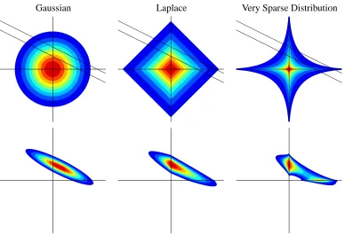
analytical treatment (see O’Hagan, 1994, Chapter 9). Such a prior does not encode sparsity. The Laplace distribution puts much more weight close to zero than the Gaussian, while still having higher probabilities for large values. The implications are depicted in Figure 1, see also Tipping (2001).
A sparsity prior embodies the bi-separation characteristic: such parameters a with many very small components at the expense of few large ones are favoured over a whose components are
Gaussian Laplace Very Sparse Distribution
Figure 1: The entries of the parameter a can be given different prior distributions. Shown above are three candidates, plotted jointly over the values of two entries: a Gaussian, a Laplace, and a “very sparse” distribution (P(ai)∝exp(−τ|ai|0.4)). We show contour plots of density functions, where areas of a specific color contain the same probability mass for each of the distributions. The upper row shows prior distributions of unit variance, together with the likelihood for a single measurement (a single linear constraint with Gaussian uncertainty). The lower row shows the corresponding posterior distributions. Whereas the Gaussian prior is spherically distributed, the other two shift probability mass towards the axes, so that more mass is given to sparse tuples (with one entry close to zero). This effect is clearly visible in the posterior distributions, being the normalised product of prior and likelihood. For the Gaussian prior, the areas close to the axes have rather low mass. In comparison, the posterior for the Laplace prior is skewed, so that more mass is concentrated close to the vertical axis. Both posteriors are log-concave and unimodal. The posterior for the “very sparse” prior shows shrinkage towards the axes even more strongly, and in terms of enforcing sparsity, this prior is preferable to the Laplacian. However, the posterior is bimodal now, suggesting two different interpretations for the single observation. The number of posterior modes can increase exponentially with the number of dimensions, so that sampling from or even representing this distribution has combinatorial complexity in general. Figure by Florian Steinke.
parameters are shrunk towards zero selectively, while a Gaussian prior leads to a more uniform shrinkage. This characteristic is embodied even more strongly in sparsity priors other than the Laplace, such as “spike-and-slab” (mixture of narrow and very wide Gaussian), Student’s t, or distributions∝exp(−| · |α),α<1, see also Figure 1. Among these, only the Laplace distribution is log-concave, leading to a posterior whose log density is a concave function, thus has a single local maximum. This simplifies and robustifies accurate inference computations significantly (see Section 3.5). For a non-log-concave prior, posteriors tend to be multi-modal, spreading their mass among many bumps, and accurate approximate inference can be a very hard problem. Furthermore, existing variational inference methods are more prone to non-robust unstable behaviour if applied to such models, and convergence or approximation errors can be hard to assess. Since we aim our method to be robust and easy to use by non-experts, we concentrate on log-concave Laplace sparsity priors in the sequel. The importance of log-concavity has been recognised in statistics and Markov chain sampling (Pratt, 1981; Gilks and Wild, 1992; Park and Casella, 2005; Lov ´asz and Vempala, 2003; Paninski, 2005), but has not received much attention so far in work on variational approximate inference.
Our decision to prefer the Laplace sparsity prior over the conventional Gaussian choice, at the expense of having to approximate inference and of introducing significant complications, is ulti-mately validated by our experimental findings, where the Laplace prior yields large improvements over the Gaussian setting (see Section 7.1). However, apart from failing to encode a sparsity bi-separation, the Gaussian prior leads to other serious artifacts in the context of experimental design with the linear model. For example, suppose we are interested in sequentially designing covariates
x for which responses u are queried (this is related to, but not the same setting we use here, see
Sec-tion 4), say by choosing a “locaSec-tion” t in a feature map x(t). It is well known and easily established that the Bayesian optimal design is independent of the response measurements we obtain along the way, it can in fact be computed beforehand. This fact seems absurd for many design problems, in-cluding ours here, pointing out a shortcoming of the model-prior combination. In the gene network identification problem (see Section 2.2 for notation), if we were to use a Gaussian prior, the poste-rior covariances would be identical for all rows of A. This means that no matter what disturbance experiments are done, the uncertainty in how gene i is influenced directly by the others, is the same for all i! Since design decisions mainly hinge on these uncertainty estimates, such artifacts due to a bad prior choice can lead to very suboptimal outcomes (see Section 7.1).
It is important to contrast our approach, and more generally the Bayesian statistical notion of sparsity, with what some maximum a posteriori (MAP) treatments of the sparse linear model are aiming to do. In the latter approach, which is very prominent in machine learning (Tibshirani, 1996; Chen et al., 1999; Peeters and Westra, 2004), the mode ˆa of the posterior P(a|X,u)is found through convex optimisation (recall that the log posterior is concave), and ˆa is treated as posterior estimate
of a. ˆa has the property that many components are exactly zero:5 the vector is sparse as such.
This is useful for applications which aim for such exact sparsity, say for reasons of algorithmic efficiency. In contrast, in the Bayesian case, the posterior mass of all exactly sparse a (at least
one component exactly zero) is zero, because the posterior has a density w.r.t. Lebesgue measure.6
Not even commonly used Bayesian estimates of a, such as posterior mean or median, are exactly sparse in general. From a Bayesian viewpoint this makes sense, since in the presence of finite data,
5. One can easily show that asσ2→0, no more than m components of ˆa can be non-zero.
one should always have some remaining uncertainty in exact values of parameters. The role of a sparsity prior in our situation is not to force many parameter values exactly to zero, but rather to enforce a clear partition into a large set of parameters which are close to zero with high (posterior) probability, and a small set which have significant mass on large values. Interestingly, following this probabilistic notion of sparsity sometimes allows to uncover sparsity in parameters of higher order that are of real interest, which is missed by MAP approaches. Our findings in Section 7.2 are a nice example of this effect.
2.2 Gene Network Identification
Measuring m-RNA expression levels for many genes in parallel is affordable and widely done today using DNA micro-arrays (DeRisi et al., 1997). One goal of such efforts is to recover regulatory networks. For example, some genes may code for transcription factor proteins, which up-/down-regulate the expression of other genes. In an active approach to network recovery, the evolution of expression levels of n genes is modeled by a system of ordinary differential equations, which is linearised at its steady state:
˙x(t) =Ax(t)−u(t) +ε(t), (3)
where x(t)is the deviation in expression from steady state, andε(t)is white noise. A is the system
matrix, whose non-zero entries represent the edges of the network. u(t) is an external control,
allowing the active user to probe the unknown A. It is generally assumed that u(t)is small enough
not to drive the system out of its linearity region. Due to the noisy environment, it is typical to restrict controls to be constant, u(t)≡u, and to measure the new steady state limt→∞x(t) (Tegn´er et al., 2003). Such disturbances may be implemented biologically using gene switches (Gardner et al., 2000), which puts further restrictions on allowable u.
The linear model of (1) captures this setup as follows. Suppose that m observations D={xi,ui}
have been made, where ui is an external control, and xi is the corresponding difference between
steady state expression levels of the perturbed and the unperturbed system. We write U = (ui)T ∈
Rm,n, X = (xi)T ∈Rm,n. We have that ui∼N(Axi,σ2I). If ai is the transpose of the i-th row of
A, this Gaussian likelihood decomposes into n factors, one for each ai. If the coefficients of A are assumed to be independent Laplacian a priori, the posterior factorises accordingly:
P(A|D) =
∏
j
P(aj|D), P(aj|D)∝N(U·,j|X aj,σ2I)
∏
iP(aj,i).
Thus, we have n independent sparse linear models, on which inference is done separately.
Since biological experiments involving gene switches are expensive and time-consuming, a key requirement is to perform with as few data as possible, which is possible if biological prior
knowl-edge is encoded in P(A). Importantly, regulatory networks are observed to be sparsely connected,
that is, plausible A are sparse, a property which is directly represented in the sparse linear model. A principled way of saving on the number of expensive experiments is optimal design, which in a special case of interest here boils down to the question: given the current posterior belief and a set
of candidate controls u∗, which of these experiments renders most new information about A? Thus,
a “value of information” is sought which can be computed for each candidate u∗without doing the
2.3 Coding of Natural Images
A second application of the sparse linear model is concerned with linear coding of natural images (Olshausen and Field, 1997; Lewicki and Olshausen, 1999), with the aim of understanding proper-ties of visual neurons in the brain. Before we describe the setup, it is important to point out what our motivation is here, since it deviates significantly from what is usually done in machine learning. One approach in theoretical neuroscience is to formulate principles which can be described reason-ably simply in mathematical terms, so that certain phenomena observed in experiments emerge if
only these principles are followed. Once such principles are established, one can think about neural
mechanisms implementing them. Also, if different principles lead to the same observed phenomena, one can plan experiments to further discriminate between them. In machine learning, the problems are known, and methods are compared with the aim of finding the best one, using an evaluation score and methodology independent of the set of methods to ensure a fair comparison. If results are not much different across methods, the most efficient one is usually preferred. In theoretical
neu-roscience,7the outcomes are known, and simple “universal” principles to explain them are sought.
Once a principle is suggested, the aim is to devise a method following that principle as closely as possible. If such a method can then successfully reproduce observed phenomena, the principle can be established. In the context here, we are interested in testing a hypothesis put forward by Lewicki and Olshausen (1999), which is formulated in Bayesian terms. We are not interested here in coding images in the best possible way, and certainly not in how to do this with the highest computational efficiency.
An image u∈Rm is modeled as u=X a+ε, where the columns of X are codebook vectors,
a∈Rnare basis coefficients, andε∼N(0,σ2I)independently. Note that codebook vectors are also
referred to as filters, or basis functions. A central assumption on a is sparsity, which is especially
important in the underdetermined (or overcomplete) regime: m<n. The Bayesian approach via
the sparse linear model (1) has been suggested by Lewicki and Olshausen (1999), where the aver-age coding cost of imaver-ages under the model is put forward as criterion for ranking different code matrices X . Their work aims to give a probabilistic interpretation to the findings of Olshausen and Field (1997). In a Bayesian nomenclature, the average coding cost is the negative log marginal like-lihood−log P(D), where P(D) =∏jP(uj), P(uj) =RP(uj|aj)P(aj)daj, and differences of these for different X are log Bayes factors. In Section 5, we show how to obtain a good approximation to
−log P(D)through EP, which can be minimised w.r.t. the code matrix X in a gradient-based way.
This general idea is proposed by Lewicki and Olshausen (1999) as well, but they use a
second-order (Laplace) approximation to−log P(D), which is not suitable in case of a Laplace prior.8 In
the earlier approach of Olshausen and Field (1997), the learning of X is driven by point estimates (or maximum a posteriori decoding), and a criterion different from the average coding cost is opti-mised. This ignores posterior uncertainty in the decodings, and requires additional renormalisation heuristics in order to learn a good code. Our approximation here implements the probabilistic hy-pothesis of Lewicki and Olshausen (1999) fairly accurately, and can therefore be used to analyse more closely which of the features found by Olshausen and Field (1997) are due to the minimi-sation of average coding cost, versus which may rather be caused by particular characteristics of their learning method. Note that maximisation of the marginal likelihood is an important empirical
7. Or, in fact, in most natural sciences, with the exception of Engineering and Computer Science.
8. The problem is that log P(aj)is not differentiable at the posterior mode ˆaj, so that the matrix B in Lewicki and
Bayesian way of estimating free hyperparameters, and Bayes factors are routinely used to compare model setups, so our approximation will be useful in other applications of the sparse linear model as well.
One of the key questions in natural image modelling is: under which conditions do basis vec-tors emerge which are spatially oriented and localised, thus show properties which have been es-tablished for the receptive fields of certain visual neurons? Given that the hypothesis of Lewicki and Olshausen (1999) is taken for granted, the sparsity hypothesis can be tested using the sparse linear model. Interestingly, other conditions brought forward (such as non-negativity) can also be dealt with in principle using the linear model, with different priors on a. Technically, non-negativity can be implemented by “cutting off” (and renormalising) a given prior density, which amounts to replacing P(ai) by 2P(ai)I{ai≥0}. Importantly, if P(ai) is log-concave, so is this modification,
because log I{ai≥0} is (generalised) concave. For example, “cutting off” the Laplace distribution
results in the exponential distribution,9which has been used in the context of image modelling by
Hojen-Sorensen et al. (2002). While exponential priors encode non-negativity and sparsity at the same time, a cut-off Gaussian P(ai) =2N(ai|0,τ˜−2)I{ai≥0}could be used to represent non-negativity alone.
2.4 Bayesian Compressive Sensing
There has been a lot of recent interest in signal processing in the problem of compressive sensing (Cand`es et al., 2006; Donoho, 2006). The idea is appealingly simple. Suppose a signal is measured and then transferred over some channel or stored on some media. The second step almost always includes lossy compression in practice, especially with signals such as images or sound, where the loss may not be perceivable. Many of today’s codes are sparse: the signal is transformed one-to-one, after which many coefficients are close to zero. These coefficients are then set to zero, and are not transmitted or stored. The first sensing (or sampling) step is traditionally done in a way which does not lead to loss of information, say by relying on the Nyquist/Shannon sampling theorem. The question of compressive sensing is whether one can sample a signal in a more efficient, but lossy way, so that the loss is part of that one encountered through subsequent compression anyway. The main attractiveness is that if a lossy compression is used, compressive sensing does not add further losses.
Although maybe not phrased in that way by much of the existing work, this is a classical problem of experimental design. An approximate Bayesian variant of compressive sensing has been proposed by Ji and Carin (2007), using sparse Bayesian learning (Tipping, 2001) to approximate the inference.
Most practical codes today are linear, in that y=Φa, where y is the signal (say, an image),Φ is
the code matrix (say, a Wavelet transform), and a are the coding coefficients. The code is designed such that a is approximately sparse, in much the same sense as elaborated in Section 2.1. Typically,
Φis one-to-one, even unitary. We then measure the signal linearly, that is, obtain u=Py+ε, where
P is a measurement matrix, u are the responses, andε is noise due to measurement errors. Here,
P∈Rm,n with m<n (the savings promised by compressive sensing). If X =PΦ, this is exactly
the setup of the linear model (1). Furthermore, the sparsity of a is encoded via a Laplace prior, motivating the sparse linear model for compressive sensing.
The measurement matrix P can be designed at will, where we are possibly limited to certain parametric families, due to constraints from the measurement architecture or (for very large n)
computational tractability (see Section 6). Anyway, we can design P row by row through an instance of standard sequential experimental design described in Section 4. This has been proposed in Ji and Carin (2007). Moreover, we can try to optimise P a priori over a large database of signals from the domain of the application, in what turns out to be an interesting variant of the image coding problem
of Section 2.3. Here, the image codeΦ is fixed, but P is to be learned.
Another point in which our approach differs from much of the existing work on compressive sensing, has to do with the sparsity prior we employ. Namely, many theoretical results have been obtained under the assumption that the signal y can be exactly sparsely coded, in that most coef-ficients in the corresponding a are exactly zero. However, in many real-world applications, this may be too strict an assumption. For example, the Wavelet transform of an image is virtually never exactly sparse, but rather features the bi-separation characteristic discussed in Section 2.1: many coefficients are very close to zero, and a subsequent quantisation leads to an image visually in-distinguishable from y. Our sparsity prior concentrates on the bi-separation characteristic, without enforcing exact sparseness, thus may be better suited to many compressive sensing applications than the requirement of exact sparsity.
Results from experiments with different variants of compressive sensing are in preparation (joint work with Hannes Nickisch) and will be presented in a later paper (Seeger and Nickisch, 2008).
3. Expectation Propagation for the Linear Model
Exact Bayesian inference is not analytically tractable for the sparse linear model. In this section, we show how to apply the recently proposed expectation propagation (EP) method (Minka, 2001b; Opper and Winther, 2000) to this problem, circumventing some caveats we have not seen being addressed before. We begin with a high-level description, filling in the details further below. In the case of EP for the sparse linear model, it turns out that some details concerning robustness are essential for obtaining a practically useful method.
In EP, we compute a Gaussian approximation Q(a)to the posterior
P(a|D)∝N(u|X a,σ2I)P(a).
Here, the likelihood N(u|X a,σ2I)is Gaussian, and it is the non-Gaussian prior P(a)which forces
us to approximate Bayesian inference. Our restriction to Gaussian Q(a)is primarily done for
prag-matic reasons, since Bayesian computations such as marginalisation and conditioning can be done analytically in this family, using standard matrix operations which can be computed robustly and efficiently. However, in our case, the Gaussian approximation can be argued for more strongly than
in many others. Namely, recall that log P(a) is concave (2). Since the likelihood is a Gaussian
function of a, the true log posterior log P(a|D)is concave as well, thus has a single mode only. If P(0)(a):=N(u|X a,σ2I)is the Gaussian likelihood (1), the true posterior is
P(a|D)∝P(0)(a)
∏
i
ti(ai), ti(ai) = ˜
τ
2e −τ˜|ai|.
We refer to the tias sites, and to P(0)as base measure. Note that the latter is not in general normal-isable.
In order to motivate EP, note that an optimal Gaussian posterior approximation Q(a) (at least
statistics. However, this would require a n-dimensional non-Gaussian integration, which cannot at present be done tractably. However, we are able to compute one-dimensional integrals involving a single non-Gaussian site ti(ai). EP makes use of this capability in an iterative fashion, in order to approximate the desired joint posterior moments. The EP posterior approximation has the form
Q(a)∝P(0)(a)
∏
i ˜ti(ai),
where ˜ti(ai|bi,πi)are Gaussian factors. Formally, one gets from the intractable P(a|D)to its Gaus-sian approximation Q(a) by replacing each non-Gaussian ti(ai) by a Gaussian counterpart ˜ti(ai).
This formal replacement introduces site parameters b,π∈Rn, and the EP algorithm is an iterative
method for adjusting these in turn.
In a single EP update, bi,πi are adjusted, while leaving all other site parameters the same.
Starting from the current Gaussian approximation Q, we compute the Gaussian cavity distribution
Q\i∝Q˜ti−1 by dividing out the site approximation ˜ti(ai), then the non-Gaussian tilted distribution ˆ
Pi∝Q\itiby multiplying in the true site ti(ai)instead, finally we update bi,πisuch that the new Q0
has the same mean and covariance as ˆPi. These single updates are iterated in some random ordering
over the sites until convergence.10Thus, EP is inherently based on the idea of moment matching. In
other words, Q0is chosen by minimising the relative entropy D[Pˆik·]over all Gaussians.
From an algorithmic viewpoint, several questions have to be addressed. First, how can we
represent the Gaussian Q(a), so that single EP updates are served well in terms of efficiency and robustness? We will see that a good representation has to allow for the rapid “random-access”
extraction of marginals Q(ai), and we have to be able to efficiently and robustly update it after a
change of bi,πi. Second, how can the mean and variance of the non-Gaussian ˆPi(ai)be computed accurately? To address these questions, we need to introduce some notation and details.
Denote the family of unnormalised Gaussian measures by
NU(z|b,P):=exp
−12zTPz+bTz
,
P being positive semidefinite. Then, P(0)(a) =NU(a|σ−2b(0),σ−2Π(0))withΠ(0)=XTX , b(0)=
XTu. The site approximations are ˜ti(ai) =NU(ai|σ−2bi,σ−2πi), so that Q is a Gaussian. In general
applications of EP, the πi can become negative, but this does not happen in the cases discussed
in this paper. We will show in Section 3.5 that for log-concave sites ti, allπi remain nonnegative
throughout the course of the EP algorithm.
Moreover, the reader may wonder why we restrict ourselves to ˜ti(ai), instead of allowing for
general site approximations ˜ti(a). Also, a careful reader may have noted that we are only concerned
about marginal distributions Q(ai) and ˆPi(ai)during an EP update at ti. Importantly, all this does not come with a loss of generality, as is shown in Section 3.1.
We initialise the algorithm with b=0 andπ=ε1,ε>0. A useful heuristic isε=τ2/2, making
sure that ti(ai) and ˜ti(ai) have the same variance initially. In the case of the sparse linear model,
the implementation of EP is complicated in a fundamental way. If m<n (underdetermined case),
if any of theπi=0, the resulting Q(a)is (in general) not a proper Gaussian either, so we have to
ensure thatπi>0 at all times. If mn, we would like to represent the posterior Q in a way which
scales with m rather than n. We address these issues below in this section.
It is important to note that EP is not merely a local approximation, in that ˜tiis somehow fitted to
tilocally. This would not be useful at all,11because posterior mean and covariance are shaped jointly
by the non-Gaussian ti and the coupled Gaussian base measure. Loosely speaking, the likelihood
couples coefficients ai, so that the intentions of the prior factors ti(ai), namely to force their
respec-tive arguments towards zero, have to be weighted against each other in a very non-local procedure.12
After each EP update, although only a single site approximation is modified, its influence propa-gates to all other sites, because they are coupled through the base measure. In fact, non-locality is a central aspect of Bayesian inference which makes it so hard to compute, and inference is particu-larly hard to do in models where strong long-range posterior dependencies are present which cannot easily be predicted from local interactions only.
Finally, would it not be much simpler and more efficient to locate the true posterior mode through convex optimisation (recall that the posterior is log-concave), then do a Laplace approx-imation there, which amounts to expanding the log posterior density to second order around the mode? Indeed, finding the mode can be done efficiently by solving a quadratic program (Tibshi-rani, 1996). General problems with this approach include that the curvature around the mode may not be characteristic of the target density, and that the mode may not be a good place to center a Gaussian approximation at. In the case of the sparse linear model, the Laplace approximation is
not even a valid option, since it is not well-defined in the presence of a Laplace prior.13 Namely,
log P(ai)does not have a curvature at ai=0. The posterior mode is guaranteed to contain at least
some zero components, so the curvature there is not defined. EP does not require P(ai)or log P(ai) to be differentiable. On models where both methods can be applied, EP tends to improve upon a Laplace approximation significantly, but is also typically more expensive (Minka, 2001a; Kuss and Rasmussen, 2005).
3.1 Overview of Algorithm
In this section, we provide a schematic overview of the EP algorithm, filling in details in the sections to come. Recall that EP iterates site updates at i∈ {1, . . . ,n}, computing Q\i∝Q˜ti−1and ˆPi∝Q\iti, then adjusting Q→Q0such that Q0has the same mean and covariance as ˆPi. Since tidepends on ai only, ˆPi(a\i|ai) =Q\i(a\i|ai), where a\i:= (aj)j6=i, thus Q0(a\i|ai) =Q\i(a\i|ai). Therefore, an EP
update automatically results in the site approximation ˜ti being a (Gaussian) function of ai only. It
also implies that in order to drive the EP update, all we need is the marginal distribution Q(ai). Just as most other variational “message-passing” approximate inference methods, EP can be seen as an iterative algorithm, improving estimates of the marginals Q(ai), i=1, . . . ,n until convergence. An EP update is local, in that its input is a marginal Q(ai) and it affects single site parameters bi,πi only. However, this globally affects all other marginals, which have to be updated through Gaussian propagation.
In common variational algorithms applied to discrete structured graphical models, such correc-tions of marginal estimates are performed by passing messages along the graph. In our case, the
11. Our experiments comparing Laplace and Gaussian priors in Section 7.1 illustrate this fact very nicely.
12. Our arguments about locality assume that a neighborhood structure can be imposed on a, say neighboring pixels in an image.
Algorithm 1 Expectation propagation algorithm for sparse linear model. Require: X , u,τ,σ2,η
b=0. π=ε1. Compute initial representation of Q
repeat
for i∈ {1, . . . ,n}(random order) do
Compute marginal Q(ai) =N(ai|hi,σ2ρi)from representation Do (fractional) EP update:(bi,πi)→(b0i,π0i)
Update representation of Q
end for
Refresh representation
until marginal estimates{Q(ai)}converged
fully coupled Gaussian factor P(0)plays the role of the graph, and the messages are replaced by a
posterior representation of Q(a) =N(a|h,σ2Σ). Just as with messages, the purpose of a
represen-tation is twofold: first, it needs to deliver mean and variance of an arbitrary marginal Q(ai)rapidly. Second, we need to be able to update it efficiently after each EP update. Our representations are given in Section 3.2, together with efficient update rules. Numerical errors can accumulate after
many updates, so the representation is refreshed (i.e., recomputed from scratch) after each O(n)
EP updates. An iteration of EP updates over all (or most of the) sites is referred to as sweep. The structure of the EP approximate inference algorithm is given in Algorithm 1.
We close this section by remarking on the stopping rule we use in our EP implementation. One could stop once the site parameters do not change significantly anymore. However, we are really interested in the marginal means and variances, which in some cases are only weakly dependent on
certain site parameters. For example, a largeπi means in general that the corresponding marginal
mean is nailed down with a small variance, and increasing πi further may have no large effect
on the marginal distribution. Let d(a,b):=|a−b|/max{|a|,|b|,10−3} and ∆i =max{d(h0i,hi),
σd(p
ρ0 i,
√ρ
i)}, where Q(ui) =N(hi,σ2ρi) and Q0(ui) =N(h0i,σ2ρ0i) are the posterior marginals
before and after an update at site i. We stop once maxi∆i for a sweep over all sites is below some
threshold.
3.2 Posterior Representation
In this section, we develop a representation of the posterior approximation Q(a) =N(h,σ2Σ)which
allows efficient access to entries of h, diagΣ(marginal moments), and which can be updated
ro-bustly and efficiently for single site parameter changes (after EP updates). In fact, we propose two different representations: a degenerate and a non-degenerate one. The former is only useful in
the underdetermined case (m<n), its updates are less numerically stable and more complicated,
but it scales as O(m2), while the non-degenerate one scales as O(n2). If mn, the degenerate
representation leads to large computational savings.
We begin with the simpler non-degenerate representation:
Σ−1=XTX+Π=LLT, γ:=L−1(b(0)+b),
whereΠ:=diagπ here and elsewhere. L∈Rn,nis the lower-triangular Cholesky factor (Horn and
is determined as hi =vTγ, ρi =kvk2, where v=L−1δi. Here, δi is the Dirac unit vector with 1
at position i, and 0 elsewhere. This costs O(n2) (single back-substitution). After an EP update
bi→b0i,πi→π0i, we have that
L0(L0)T=LLT+ (π0i−πi)δiδTi , L0γ0=Lγ+ (b0i−bi)δi.
L0,γ0 are computed from L,γusing a Cholesky rank one update (downdate) for positive (negative)
π0
i−πi. This can be done in O(n2), we use a modification of theLINPACKroutinesdchud,dchdd
(Dongarra et al., 1979), see Seeger (2004) for details. The update (downdate) is not done if|π0i−πi|
is too small. The reader may wonder why we do not represent and update Σ directly, using the
Woodbury formula (see below). However, this would be numerically less stable than the Cholesky representation suggested here, and the operation count is the about the same.
In the underdetermined case m<n, another degenerate representation can be used, which leads
to large savings if mn. We noted in Section 3 above that Q is well-defined only if allπi>0. For
numerical stability (with the degenerate representation), we require thatπi≥κat all times, where
κ>0 is a small constant (we useκ=10−8presently). This constraint is enforced in all EP updates. We can use the Woodbury formula (Henderson and Searle, 1981) in order to write
Σ= XTX+Π−1
=Π−1−Π−1XT I+XΠ−1XT−1
XΠ−1.
We represent this via the lower-triangular Cholesky factor L in
LLT =I+XΠ−1XT.
Furthermore, letγ:=L−1XΠ−1(b(0)+b), whence
h=Σ(b(0)+b) =Π−1b(0)+b−XTL−Tγ
,
thus both h andΣare represented by L,γ. For not too smallκ, this representation is numerically
stable. The marginal Q(ai)is obtained asρi=π−i 1(1−π−
1
i kvk2), hi=π−i 1(b
(0)
i +bi−vTγ), where
v :=L−1x with x=X·,i. After an EP update bi →b0i,πi →π0i, the representation is modified as follows. Let∆1:= (b(i0)+b0i)/π0
i−(b
(0)
i +bi)/πi,∆2:= (π0i)−1−π−i 1. We have that
L0(L0)T=LLT+∆2xxT, L0γ0=Lγ+∆1x.
Just as above, L0,γ0can be computed from L,γas a Cholesky rank one update/downdate, at the cost
of O(m2). We do not modifyπ
iand the representation if|∆2|falls below some small threshold. All in all, we can use a representation of Q whose size, as well as cost of a single site update,
is quadratic in the smaller of n and m. Beware that L,γhave different definitions in the two cases.
Note that we can also use the non-degenerate representation in the case m<n. In general, the
non-degenerate representation leads to more numerically stable computations (supposedly because
the Woodbury formula is not used), which are in fact more efficient in practice once m≈n/2.
We recommend to use the degenerate representation only if significant computational savings are observed in practice.
In some experimental design applications, such as gene network identification considered here,
3.3 The EP Update
An EP update works by matching moments between a tilted and the new posterior distribution. For an update at site i, we require the marginal Q(ai) =N(hi,σ2ρi) only, which is obtained from the
Q representation. The moment matching requires the computation of Gaussian expectations with ti(ai), a univariate quadrature which in general is not an analytical computation.
If Q\i(ai) =N(h\i,σ2ρ\i), we have that
ρ\i=
ρi 1−ρiπi
, h\i=hi−ρibi
1−ρiπi
.
If the degenerate representation is used, it is more stable to compute the cavity marginal directly. Namely, if v :=L−1X
·,i, thenρ\i=kvk−2−π−i 1and h\i= (b
(0)
i −vTγ)/kvk2+bi/πi.
Next, we need to compute mean and variance of ˆPi(ai) =Zi−1Q\i(ai)ti(ai), which we do as
de-scribed in Seeger (2003), Appendix C.1.3. Note that Zi = EQ\i[ti(ai)], and define βi :=
(d log Zi)/(dh\i), νi :=−(d2log Zi)/(dh2\i). The concrete computation of βi,νi (or equivalently,
of the first and second moment of ˆPi(ai)) can be done analytically for Laplace sites, but is not
straightforward due to issues of numerical stability, it is described in Appendix A. Then, the new site parameters are given by
π0 i=
σ2ν
i 1−σ2ν
iρ\i
, b0i=σ
2(β
i+h\iνi) 1−σ2ν
iρ\i
.
We show in Section 3.5 thatνi≥0, thusπ0i≥0, due to the log-concavity of ti. Ifπ0i<κand the degenerate representation is used, we setπ0i=κ.
The numerical difficulties with the EP update for Laplace sites are remarkable, given that no such problems occur in several other EP applications, for example Gaussian process classification (GPC) with probit or logit noise (Minka, 2001b; Opper and Winther, 2000; Lawrence et al., 2003), where less careful implementations still work fine, and even approximate Gaussian quadrature can be used. Several early attempts of ours led to complete failure of the algorithm on realistic data (in the underdetermined case), motivating the fairly elaborate solution in Appendix A. While we cannot offer a firm explanation for this yet, our intuition is that the effect of Laplace prior sites on the posterior is much stronger, trying to emulate the essentially discrete feature selection process in a “unimodal” manner. Our findings also shed some sceptical light on proposals to implement a
generic toolbox for EP, applying Gaussian quadrature14 to do EP updates for general sites (Zoeter
and Heskes, 2005). In the gene network identification application, we ran into problems of numer-ical instability coming from the combination of Laplace sites with very underdetermined coupling
factors P(0). We suspect these problems are inherent, and in our case could be handled only by
considering a modification of EP, as discussed just below.
3.3.1 FRACTIONALEP UPDATES
We just mentioned the numerical difficulty of doing EP updates with Laplace sites in the strongly
underdetermined case m<n. A frequent cause of numerical problems with EP is sloppiness in
the implementation. For example, representation updates based on the Woodbury formula are a frequent source of accumulation of round-off and cancellation errors (see Section 3.2). The EP
update with Laplace sites is quite difficult to do in a stable way (see Appendix A).15However, even
using all these careful measures did not allow us to run standard EP on many of the gene network identification problems of Section 7.1 or on a fraction of the image coding problems of Section 7.2. We think that these stability problems of EP are inherent for some tasks, giving some motivation below. Fortunately, EP can be modified to use fractional updates, which in fact counter exactly the numerical problems we face. While fractional EP has been suggested as alternative to standard EP (Minka, 2004), its role for circumventing stability problems has not been noted so far to our knowledge.
Recall from Section 3 that if we set all or most of the πi=0 in the underdetermined case, the
variance of most marginals Q(ai)is infinite. We face this problem by ensuring that πi≥κat all
times. Still, at least for some updates, the cavity marginal variance of Q\i(ai) is huge. This is
because we divide through the site approximation ˜ti(ai), whoseπi ≥κ keeps the variance small.
The variance is not infinite due to the effect of the otherπj ≥κand the coupling through P(0), but in many underdetermined situations, this coupling is weak. We then try to do an EP update based on a very wide cavity distribution Q\i(a
i)and a quite narrow site ti(ai)(enforcing a strong sparsity constraint requires a rather largeτ). This is inherently difficult to do.
It would be better to make Q\i(ai) narrower and ti(ai) wider, which is exactly what happens in fractional EP updates. Here, we obtain Q\i(ai) by dividing out only a fraction of ˜ti(ai), and
ˆ
Pi(ai)by multiplying with only a fraction of ti(ai). This idea is fairly natural, simply imagine the
sites being replicated q times, then taken to the power ofη=1/q to obtain the original setup. The
only difference to standard EP is that we tie the parameters of the corresponding fractional site approximation replicas. Of course, the idea is not limited to rational fractions. Some extensions and theory of this method are discussed by Minka (2004). Another view on fractional EP is that
projections from standard EP’s ˆPi to Q0 are done based not on the relative entropy (see Section 3),
but on anα-divergence depending on the fraction.
For the fraction parameter η∈(0,1], let Q\i ∝Q˜ti−η and ˆPi ∝Q\itiη. We choose the new site parameters b0i,π0i such that the moments of ˆPi and Q0 match. This can be incorporated into the derivations above by setting ˜bi=ηbi,π˜i=ηπi, and ˜τ=ητ. The cavity moments are computed as
ρ\i=
ρi 1−ρiηπi
, h\i=
hi−ρiηbi 1−ρiηπi
.
For the degenerate representation, a direct computation may be more stable:
ρ\i=π−i 1
R
1−ηR, h\i=π
−1
i
b(i0)−vTγ
1−ηR +bi
!
, R=1−π−i 1kvk2.
We then compute ˜b0i,π˜0i as above, using ˜τ=ητ instead of τ in the Laplace site, so that ˆPi and
∝Q\i˜ti(·|˜b0i,π˜0i)have the same moments. Fractional updates are easily implemented for sites ti(ai|τ) with some hyperparameterτ, such that ti(ai|τ)η=ti(ai|ητ). The Laplace site is of this kind, if the normalisation constant ofτ/(2σ)is dropped (it does not affect mean or variance of ˆPi). Note that in
general, tiηis log-concave if ti is. Finally, the site parameters are updated as
b0i= (1−η)bi+˜b0i, π0i= (1−η)πi+π˜0i,
upon which ˆPiand the new Q0have the same moments.
Another idea of making EP run smoother on hard problems is damping (Minka, 2001a). There, the full standard EP update is computed, but the site parameters are updated to a convex combination of old and proposed new values. This addresses a quite contrary problem to ours here. Damping is useful if EP update computations are stable, but lead to an improper new posterior, or the prop-agation of the updated information fails. If EP is viewed as finding a saddle point of a free energy approximation (Opper and Winther, 2005), damping can be understood as a step-size rule within this process. It slows down convergence in general in situations where EP without damping works fine, but the fixed points are not altered. Our problem is not solved by damping, since proposed new values for the site parameters cannot even be computed.
Finally, the reader may wonder whether the problems with standard EP are due to a bad initial-isation of the site parameters. While we have not analysed it in all details, we think the problem is inherent. For example, we tried to run fractional EP to convergence, then start standard EP (with
η=1) from the fractional fixed point. On critical cases, this fails about as fast as if started in the usual way, often in the first sweep of standard EP.
3.4 Inclusion of a New Point
Suppose we would like to operate inference in the sparse linear model in a sequential manner, in
that new data points (x∗,u∗) become available over time. This is the case in sequential design
applications, since single experiments result in new measurements. In this section, we show how the EP posterior representation is updated once a new point(x∗,u∗)is added to the current data set
D. The inclusion of(x∗,u∗)works in two stages. First, the Gaussian base measure is modified in order to incorporate the new point. Second, EP updates are done until convergence. The mechanics of the latter have been described above, so we can concentrate on the first stage here.
For the non-degenerate representation, let v :=L−1x∗. The change of b(0) results in ˜γ=γ+ u∗v. Since L0(L0)T =LLT+x
∗xT∗, L0,γ0 is obtained from L,γ˜ by a rank one Cholesky update (see Section 3.2). The cost is O(n2).
For the degenerate representation, let X0= (XT,x
∗)T∈Rm+1,nand u0= (uT,u∗)T∈Rm+1. Since
b(0)=XTu, we have that b(0)0=b(0)+u∗x∗. Let l :=L−1XΠ−1x∗. Then, ˜γ=γ+u∗l incorporates
the update of b(0). Next, LLT grows by a row/column((Ll)T,1+xT
∗Π−1x∗)T. Therefore, L0,γ0are
obtained from L,γ˜by a Cholesky extension, as described in Seeger (2004). The cost of the inclusion
is O(m2).
3.5 Some Consequences of Log-concavity
A nonnegative function f(x)is log-concave if
f(λx1+ (1−λ)x2)≥ f(x1)λf(x2)1−λ
for all x1,x2, andλ∈[0,1]. f(x) is log-concave iff log f(x) is concave as a generalised function,
which can take on the value−∞, see Boyd and Vandenberghe (2002), Sect. 3.5. We call a
Gaussians are clearly log-concave, so models of the sort considered here are log-concave if the sites are (products of log-concave functions are log-concave). For example, Laplace sites ti(ai)are log-concave, while Student’s t sites are not. A direct consequence is that for log-concave sites, the posterior is log-concave, so its unique mode can be found by convex optimisation. Log-concavity is stronger than unimodality though. For example, all upper level sets (areas enclosed by con-tours) of the posterior are convex sets. Intuitively, log-concave distributions are “simple”, although strong consequences of this fact for variational approximate inference methods are not known to
our knowledge.16 Our main result is the following theorem.
Theorem 1 Let EP be applied to a model with true posterior of the form P(a|D)∝P(0)(a)
∏
i
ti(ai),
where P(0)(a)is a joint unnormalised Gaussian factor, and the sites ti(ai)are log-concave. Suppose
the site parametersπi are initialised to non-negative values. Then, all EP updates are computable
(in exact arithmetic), and allπi remain non-negative throughout.
The proof is given in Appendix A.1. The theorem holds just as well for general sites ti(a)
with corresponding site approximations ˜ti(a) =NU(σ−2bi,σ−2Πi), if “πi≥0” is replaced by “Πi positive semidefinite”. It hinges on a fundamental marginalisation theorem for log-concave
func-tions due to Pr´ekopa, see Bogachev (1998). Namely, suppose that f(x,y) is jointly log-concave
in(x,y), x∈Rp, y∈Rq. ThenR
f(x,y)dy is log-concave in x. Theorem 1 implies that EP can
be implemented in a numerically stable way. Namely, the non-negativity of allπi ensures that the
representations introduced in Section 3.2 can be updated in a stable manner. The situation for some applications with non-log-concave sites is much less satisfactory. It is usually not possible to keep
allπi positive anymore, without making significant approximation errors (Minka, 2001a). Full EP
updates lead to erratic behaviour or cannot even be done, and damping has to be used, leading to
slower convergence. Negative entries πi can lead to very ill-conditioned Cholesky factors in the
representations, resulting in large errors at each update.
Our theorem also implies that for applications where EP is started withπ=0, for example
Gaus-sian process classification, we have that the entropy H[Q]of the posterior decreases monotonically
during the first sweep. Namely, the entropy is log|Σ|up to constants, which is decreasing in every
singleπi. Minka (2001a) notes that the first sweep of EP is equivalent to a method called assumed
density filtering (Kushner and Budhiraja, 2000), so our theorem has implications for this method as
well.17
Another interesting consequence of log-concavity holds for the sparse linear model, independent of whether EP is used for approximate inference or not. It serves to motivate the parameterisation of the Laplace sites (2) in terms of ˜τ=τ/σ. Up to additive constants, log P(u,a)has the form
(2m+n)logσ−1−1
2ku/σ−X a/σk
2 −τ
∑
i
|ai/σ|,
16. In contrast, MCMC sampling from log-concave distributions has been proven to be computationally efficient (Lov ´asz and Vempala, 2003).
which is jointly concave in(φ,σ−1), whereφ:=a/σ. This fact has been noted in Park and Casella
(2005). In fact, even P(u,a)σis log-concave in(φ,σ−1), since 2m+n≥1. The marginal likelihood
P(u) is a crucial criterion when it comes to hyperparameter optimisation or Bayesian tests (see
Section 5). Now,
P(u) = Z
P(u,a)da= Z
P(u,a)σdφ,
and by the marginalisation theorem, P(u) is log-concave in σ−1. This implies that if all other
hyperparameters are fixed, the empirical Bayesian maximisation of log P(u)w.r.t. the noise variance
σ2is in fact a convex problem with a unique solution. Unfortunately, this property does not extend
to other hyperparameters such asτor X . On a practitioner’s level, it is interesting to relate this fact to a scheme mapping out the entire regularisation path of Lasso (or, equivalently, an SVM) (Hastie et al., 2004). In either case, adjusting one hyperparameter trading off prior and likelihood given all
others is shown to be simple. Here, as there, this gives some reassurance ifσ2is adapted along with
other parameters (see Section 7.2).
We close this section by some technical side comments for readers interested in details, all others
may skip this paragraph. We require results from Section 5. We just showed that the exact log P(u)
is concave inσ−1, but how about the EP approximation of this quantity, called L in Section 5? To
answer this question, we first have to establish that L is well-defined and continuous as a function
of σ2 in the first place. Now, L is defined in terms of the site parameters at convergence, and
the EP algorithm has not been proven to always converge uniquely. Opper and Winther (2005)
show that L is a proper approximate free energy as function of b,π, but the site parameters at
convergence are only a saddle point thereof. Using tools such as the implicit function theorem,
one can argue that L(σ2)is well-defined across some range, but does this hold globally across all
σ2? If the dependence of the site parameters onσ2 is ignored locally, then L is log-concave in
σ−1, following similar arguments as above. We know from Section 5 that for computing the first
derivative w.r.t.σ2, the site parameters can be assumed constant, but this is not true in general for the second derivative (which would characterise concavity). Clearly, there is more work needed to gain a better understanding of such properties of the implicitly defined EP approximate free energy
L.
4. Sequential Optimal Design
The role of sequential optimal design18for saving on expensive experiments has already been
moti-vated in Section 2. The topic is well-researched in classical and Bayesian statistics (Fedorov, 1972;
Chaloner and Verdinelli, 1995). A variant is known in machine learning as active learning19(Seung
et al., 1992). We follow MacKay (1991) here, whose setting is closest to ours.
In the sparse linear model, a typical design problem can be formulated as follows. Given a set
of candidate points x∗, at which of these should a corresponding target value u∗be sampled in order
to obtain as much new information about the unknown a as possible? Assuming (for the moment)
that u∗ is known for a x∗, natural scores quantify the decrease in posterior uncertainty or gain in
18. Optimal design is a fixed term in statistics for a methodology, in which designs are optimised. We have no intention of claiming that any of the methods presented here solve problems in an optimal way, in fact they usually do not. In the context of this paper, optimal design and experimental design mean the same thing.