Some Greedy Learning Algorithms for Sparse Regression and
Classification with Mercer Kernels
Prasanth B. Nair [email protected]
Arindam Choudhury [email protected]
Andy J. Keane [email protected]
Computational Engineering and Design Center School of Engineering Sciences
University of Southampton, Highfield Southampton SO17 1BJ, United Kingdom
Editors: Carla Brodley and Andrea Danyluk
Abstract
We present some greedy learning algorithms for building sparse nonlinear regression and classifi-cation models from observational data using Mercer kernels. Our objective is to develop efficient numerical schemes for reducing the training and runtime complexities of kernel-based algorithms applied to large datasets. In the spirit of Natarajan’s greedy algorithm (Natarajan, 1995), we it-eratively minimize the L2loss function subject to a specified constraint on the degree of sparsity
required of the final model until a specified stopping criterion is reached. We discuss various greedy criteria for basis selection and numerical schemes for improving the robustness and computational efficiency. Subsequently, algorithms based on residual minimization and thin QR factorization are presented for constructing sparse regression and classification models. During the course of the incremental model construction, the algorithms are terminated using model selection principles such as the minimum descriptive length (MDL) and Akaike’s information criterion (AIC). Finally, experimental results on benchmark data are presented to demonstrate the competitiveness of the algorithms developed in this paper.
Keywords: Sparse Learning Machines, Kernel Methods, Greedy Algorithms, Regression,
Classi-fication, Model Selection.
1. Introduction
We consider the supervised learning problem of constructing a regression or a classification model using observational data
D
:= (xi,y(xi)),i=1,2,...,m, where xi ∈Rp denotes the input vectorand y∈Ror{−1,1} denotes the target to be approximated. In particular, we focus on models of the form ˆy(x) =∑nj=1αjk(x,x∗j), where{x∗j}nj=1⊆
D
. Further, k(x,xi)is a Mercer kernel (Vapnik,1995), i.e., the Gram matrix K∈Rm×mwith elements Ki j=k(xi,xj)is symmetric positive definite
(SPD). We compactly denote the weight vector as α={α1,α2,...,αm} ∈Rm, and the vector of
targets as y={y(x1),y(x2),...,y(xm)} ∈Rm. The structure of the model considered here is typical
of that encountered in regularization networks and support vector machines (Evgeniou, Pontil and Poggio, 2000).
be computed by solving Kα=y. As a consequence the resulting model behaves as an interpolator. In
contrast, when the targets are corrupted by noise, y=Kα+η, whereη∈Rmdenotes noise typically assumed to be
N
(0,σ2). Hence, one needs to solve (K+σ2I)α=y to compute the regularizedweight vector. Note that computation of the weight vector for both cases would require
O
(m2)memory and
O
(m3)operations, which would clearly be prohibitive for large datasets.1.1 Sparse Approximations
In the present paper, we use the term sparse to denote models of the form ˆy(x) =∑nj=1αjk(x,x∗j),
where{x∗j}nj=1⊆
D
and n<m. In other words, given a dictionary of Mercer kernels centered oneach training data point (i.e., k(x,xi),i=1,2,...,m), the learning algorithm chooses only a subset
of the kernels in the final model. Such a solution naturally arises when a support vector machine (Vapnik, 1995) or the relevance vector machine (Tipping, 2001) is applied to approximate the target. However, when the L2loss function is minimized, the resulting weight vector may not be sparse even
in the presence of regularization. In this paper, we present greedy learning algorithms for computing sparse approximate solutions to the L2 loss minimization problem.1 The motivation for this is to
exploit fast algorithms for matrix computations and also to investigate the generalization ability of sparse approximate solutions to the L2loss function.
In particular, we consider the problem when the memory requirements and computational costs are sought to be minimized by solving the overdetermined least-squares problem: min||Knαn−y||2, where Kn∈Rm×n is a rectangular matrix formed by choosing a subset of the m columns of the original Gram matrix andαn∈Rn denotes the truncated weight vector. Note that since K is SPD,
Knhas full column rank. This approach intrinsically leads to a sparse model since n<m and hence
only a subset of the training data is employed in the final model. In addition, this approach requires only
O
(mn) memory andO
(n3) operations for computing the weight vector. Further, the sparse model requires onlyO
(n)operations for predicting the target at a testing point.Since the empirical/training error of the sparse approximation becomes ||Knαn−y||2=ε>0 for n<<m, such a model may also be referred to as a sparse approximate interpolator. Recently,
Natarajan (1999) presented a theoretical justification for regularization via sparse approximate inter-polation. It was shown that interpolation error (ε) and noise in the target vector y will tend to cancel out ifεis chosen a priori to be the noise intensity. Natarajan’s sparse approximation problem can be formulated as: find a sparse vectorα∈Rmsuch that||Kα−y|| ≤ε. Alternatively, this problem may be interpreted as a subset selection problem of the form: find n columns of the matrix K such that min
αn ||K
nαn−y||2≤ε.
Clearly, choosing n columns out of m possible choices involves a combinatorial search over an mCn space. As shown by Natarajan (1995), this problem is NP-hard, and we have to resort to
suboptimal search schemes to ensure computational efficiency. Note that the problem statement considered here appears in the literature in different guises, for example, basis selection methods, basis pursuit, matching pursuits (Chen, Donoho, and Saunders, 1998), and sparse approximate in-verse computation (Chow and Saad, 1997; Grote and Huckle, 1997).
1.2 Outline of the Paper
In this paper, we present some greedy learning algorithms for constructing sparse nonlinear re-gression and classification models with Mercer kernels. In particular, our focus is on selecting an optimal subset from a dictionary of Mercer kernels for function approximation and classification. We examine the computational properties of existing greedy algorithms in the domain of signal pro-cessing and preconditioned iterative numerical methods. Drawing on developments in these fields, we derive iterative algorithms based on residual error minimization and thin incremental QR fac-torization for building sparse regression and classification models. The MDL principle and AIC are employed as termination criteria to determine the optimum level of sparsity. We show that the present algorithms are computationally more efficient and require significantly less memory than existing greedy algorithms. Numerical studies on some popular benchmark problems also suggest that our algorithms lead to models with good generalization abilities.
This paper is organized as follows: In Section 2, we present some relevant background on greedy algorithms. Section 3 outlines various considerations involved in developing robust greedy algorithms with modest memory requirements and low computational cost. Section 4 presents a residual minimization technique and a greedy thin incremental QR factorization scheme for updat-ing the weight vector durupdat-ing the iterations of a greedy algorithm. In Section 5, we outline stoppupdat-ing criteria based on the principles of MDL and AIC to construct parsimonious models. Section 6 presents experimental investigations on a synthetic dataset as well as some real-world datasets, and Section 7 concludes the paper and discusses future directions of research.
2. Preliminaries
The greedy algorithms in the literature can be broadly classified into sequential forward greedy al-gorithms (Mallat and Zhang, 1993; Natarajan, 1995; Grote and Huckle, 1997; Smola and Bartlett, 2001; Vincent and Bengio, 2001; Friedman, 2001), backward greedy algorithms (Couvreur and Bresler, 1999), and mathematical programming approaches (Chen, Donoho, and Saunders 1998; Girosi, 1998). In general, sequential forward algorithms are computationally cheap and tend to have modest memory requirements. In contrast, backward greedy algorithms are computationally much more expensive since the full-order Gram matrix is factorized prior to iteratively annihilating columns which lead to minimal increment in the residual error (Couvreur and Bresler, 1999). From a theoretical point of view, backward algorithms have provable convergence properties. In con-trast, forward algorithms offer no such known guarantees. Mathematical programming approaches to sparse approximation attempt to reduce the L0norm of the weight vector by minimizing an
ap-proximation to it; see, for example, Girosi (1998) and Chen, Donoho, and Saunders (1998). The computational cost associated with this class of algorithms also tends to be much higher than se-quential forward greedy approaches.
There exist intimate connections between sequential forward greedy techniques and boosting al-gorithms (Freund and Schapire, 1996). More specifically, gradient boosting alal-gorithms (Friedman, Hastie and Tibshirani, 2000; Friedman, 2001) can be interpreted as a generalization of forward greedy algorithms to minimize general loss functions. A theoretical analysis of the L2boost
proce-dure for regression and classification problems has been recently presented by B ¨uhlmann and Yu (2001). It was shown both theoretically and empirically that the performance of L2boost is
functions2selected at an earlier stage are not updated. In contrast, our approach is a stepwise proce-dure where backfitting is carried out at each iteration to adjust the weights of all the basis functions selected so far.
We mention that efficient learning with kernels has been the focus of research in a number of recent articles. Of these, the ones that are closest in spirit to the present work, focus on obtaining reduced order approximations for the Gram matrix either greedily (Smola and Sch¨olkopf, 2000) or through random subsampling (Williams and Seeger, 2001). However, the techniques presented in this work have in general more attractive computational and storage properties as compared with the above schemes and also show more promise for use as an off–the–shelf tool.
In the present paper, we restrict our discussion to sequential forward greedy algorithms applied to minimization of the L2 loss function. We present below a brief overview of one such
repre-sentative sequential forward greedy scheme, viz. Natarajan’s algorithm. A comparison study by Adler, Rao and Kreutz-Delgado (1996) has shown that this algorithm generally performs better than other algorithms in the literature. Hence, we will benchmark the numerical schemes developed in the present research against Natarajan’s algorithm. Note that Natarajan’s algorithm is equivalent to the orthogonal least-squares (OLS-RBF) technique presented earlier by Chen, Cowan, and Grant (1991) for constructing parsimonious radial basis function networks. A detailed investigation of the OLS-RBF algorithm and its application to machine learning problems can be found in Vincent and Bengio (2001).
The following notation has been used throughout this paper; we denote the inner product be-tween two vectors as(x,y) =xTy. ej∈Rmis used to denote the j-th unit vector. We employ “colon”
notation of the form K(:,I)∈Rm×pto denote the matrix formed using column indices chosen from the set I of cardinality p. We will refer to the ip-th column of the Gram matrix K∈Rm×m by kip ∈Rm.αj will be used to refer to the j-th element of the vectorα. Further, the superscript pwill
be used to denote the iteration index.
2.1 Natarajan’s Algorithm
Natarajan’s algorithm (Natarajan, 1995) consists of recursively choosing and modifying the columns of K in an iterative fashion so as to maximally reduce the L2 norm of the residual error vector r=y−Kα. Let Kp−1∈Rm×(p−1) denote the matrix of p−1 columns chosen till the(p−1)-th iteration, and let Ip−1represent the set of corresponding column indices in Kp−1. The p-th iteration then involves choosing a previously unselected column kip from K such that ||r||2 is maximally
reduced.
The initialization step of Natarajan’s algorithm involves normalizing the columns of K and setting the initial residual to y, i.e., r0=y. Let ˜K denote the normalized Gram matrix. The steps
involved at the p-th iteration are shown below:
ip = arg max j6∈Ip−1|(˜k
p−1 j ,r
p−1)| (1)
Ip ← [Ip−1,ip]
rp ← rp−1−(˜kipp−1,rp−1)˜kipp−1 (2) ˜kp
j ← ˜k p−1 j −(˜k
p−1 ip ,˜k
p−1 j )˜k
p−1
ip , ∀ j6∈I
p (3)
˜kp
j ←
˜kp j ||˜kp
j||2
∀ j6∈Ip (4)
Note that once a suitable index is selected according to (1), the residual is updated accordingly (2) and all the unselected columns reoriented (3) and normalized (4). The final weight vectorαn∈
Rnafter n iterations can be computed by solving the least squares problem minkKnαn−yk2, where Kn∈Rm×ndenotes the rectangular Gram matrix formed using the indices in In.
It can be noted from (1) that the index selection criterion is applied only to previously unselected columns. Hence, this scheme does not suffer from the recycling problem encountered in greedy algorithms such as basis matching pursuit (Mallat and Zhang, 1993) and the scheme of Schaback and Wendland (2000). Hence, Natarajan’s algorithm is also referred to as order recursive matching pursuit (ORMP).
Further, the following theorem guarantees a sparse weight vector at the end of the ORMP itera-tions when an upper boundεon the norm of the residual is specified as the termination criterion.
Theorem 1[Natarajan, 1995]: The number of non-zero elements in the weight vectorα∈Rmis at most
r≤ d18Opt(ε 2)kK
−1k2 2ln(
kyk2
ε )e
where Opt(2ε)denotes the fewest number of non zero entries over solutions that satisfykKα−yk2≤
ε
2.
A more detailed theoretical analysis of the convergence rate of a class of greedy algorithms has been recently presented by Zhang (2001). This analysis shows that the residual error is reduced by
O
(1/p)at the p-th iteration.The major computational cost incurred in ORMP is in step (1) and the column update in step (3), which has to be undertaken for all the unselected columns left at each iteration.3 It can be noted that
O
(m2) operations are required at each iteration. For large datasets, this could significantlyincrease the training time. Further, the ORMP algorithm requires the computation and storage of the full-order Gram matrix. Similar computational cost and memory requirements also arise in the case of the OLS-RBF algorithm and L2Boost procedures applied to a dictionary of Mercer kernels.
In contrast, the techniques presented in this paper have much lower memory requirements, and are generally faster while achieving comparable (or better) generalization performances.
3. Structure of Greedy Algorithms
In this section, we present an overview of the structure of greedy algorithms developed in this paper. A fundamental component of a greedy algorithm is the choice of criterion employed to select a new
column at each iteration. Once a new column is chosen, it is necessary to update the weight vector
αand the residual error vector, r=y−Kα. Further, to ensure robustness, we also need to allow the flexibility of dropping a previously chosen column. We discuss next various considerations involved in designing a computationally efficient greedy algorithm.
3.1 Criteria for Basis Selection
This crucial step involves the use of a criterion for deciding which new column should be chosen at the current iteration. Clearly, it would be preferable to choose the column which leads to the greatest reduction in the residual error. One way to achieve this would be to examine the current residual (r), and search for the entry with highest absolute value. Since, we are working with a dictionary of Mercer kernels, the Gram matrix K is SPD and consequently, the residual r provides the direction of maximum decrease in the cost function 0.5αTKα−αTy. Assuming that the residual error vector
is implicitly computed at each iteration, this criteria would incur negligible computational cost. Further, to implement this criterion, one only needs to store up to n columns of the Gram matrix, where n is the maximum number of iterations.
In line with Natarajan’s algorithm, an alternative approach would be to work with the residual corresponding to the normal equations,4 i.e., KTKα=KTy. However, this involves
O
(m2)opera-tions to compute the normal residual KTr, as well as the requirement of computing and storing the
full-order Gram matrix.
A different criterion was proposed by Huckle and Grote (1997) in the context of constructing sparse approximate inverse preconditioners. They suggested that by solving a sequence of one-dimensional minimization problems (over the columns not yet selected), the column which leads to greatest reduction in the residual can be chosen. To illustrate this, let Ip−1denote the indices of the columns chosen at the(p−1)th iteration. A new column can then be selected at iteration p by solving(m−p+1)one-dimensional minimization problems of the form
min
µj,j6∈Ip−1
krp−1+µjKejk2
The solution of this minimization problem turns out to be
µj=−
(rp−1,Ke j) (Kej,Kej)
For each j, the L2norm of the new residual rp−1+µjKejcan be written as
ρ2
j=krp−1k22−
(rp−1,Kej)2 (Kej,Kej)
Note that solving all the (m−p+1) minimization problems would require the computation and storage of the full-order Gram matrix. Recently, Smola and Sch¨olkopf (2000) proposed a gen-eral probabilistic approach for sparse approximation. The success of their approach (cf. Smola and Bartlett, 2001) suggests that, in practice, by solving around 60 one-dimensional minimization problems for randomly chosen column indices (where, column index j 6∈Ip−1), columns which
are probabilistically in the top 95th percentile can be chosen. Such a probabilistic approach may hence lead to a significant reduction in the number of one-dimensional minimization problems to be solved. However, in the present paper, we pursue the simpler criterion which involves searching for the index with the largest absolute value in r.
3.2 Updatingαand r
Once a new column is selected, we need to update the weight vectorαand the residual error vector
r. Further, it is desirable to do this step with minimal computational effort.
Smola and Bartlett (2001) update the weight vector by explicitly updating the inverse of E(:
,Ip)TKE(:,Ip),5 when an additional column is added at each iteration. However, such explicit updates when computed frequently could lead to numerical instabilities due to round-off error accu-mulations. Note that it is also possible to modify many existing iterative schemes based on Krylov subspace methods (Chow and Saad, 1998) for solving a system of linear algebraic equations to compute sparse approximate solutions. For example, by enforcing sparsity on the Krylov subspace
{r,Kr,K2r...}, the resulting approximation toαwill also be sparse.
In the present research, we consider two fast numerical schemes which are expected to be nu-merically more stable. The first scheme described in Section 4 is an iterative scheme based on residual error minimization. The second scheme presented in Section 5 uses a thin incremental QR factorization update scheme. Both these schemes only incur
O
(mn) operations at each iteration of the greedy algorithm.ALGORITHM 1: Exchange Algorithm 1. s←arg min
j∈Ip|r p j|
2. l←arg max j6∈Ip|r
p j|
3. γ← (rp+α
p sKes,Kel)
(Kel,Kel)
4. ˜r←rp+αspKes−γKel
5. If||˜r||<||rp||then
αp s ←0
αp l ←γ rp← ˜r
Ip←[Ip\s,l] End if
3.3 Exchange Algorithm
Most forward greedy algorithms in the literature do not allow for the possibility of annihilating a column once it has been chosen. Hence, for some problems, a forward greedy algorithm which makes a myopic choice at an early iteration may end up choosing an exorbitant number of additional columns to compensate for the previous choice. To circumvent this possibility, we include a step which allows for the flexibility of dropping a column based on the progress of the iterations. There are many possibilities for achieving this. For example, one could integrate backward (Couvreur
and Bresler, 1999) and forward greedy algorithms to combine the robustness of the former and the computationally efficiency of the latter approach. However, here we pursue a simpler approach motivated by the algorithm presented by Chow and Saad (1997) for computing sparse approximate inverses.
The basic idea is to drop the index for which|r|is lowest (say s∈Ip) in favor of a previously unselected column index with the largest value in|r|(say l6∈Ip), if this leads to a reduction in the current residual. To check whether this exchange strategy will lead to a lower residual, we need to solve the one-dimensional minimization problem:
min
γ ky−K(α
p−αp
ses+γel)k2
The solution of this minimization problem is given by
γ= (rp+α p
sKes,Kel) (Kel,Kel)
whereαpand rpdenotes the weight vector and residual error at iteration p, respectively.
The steps of the exchange algorithm are summarized in Algorithm 1. Note that the operation Ip\
s indicates the process of removing the index s from the set Ip. It can be seen that the exchange step will cost
O
(m)additional operations at each iteration of the greedy algorithm. A similar exchange strategy can be coupled to a thin incremental QR factorization scheme as discussed in Section 5.4. Incremental Greedy Learning Algorithms
Having outlined the essential building blocks of greedy learning algorithms for minimizing the L2
loss function, we present two numerical schemes. First, we present a minimal residual iteration scheme for updatingαand r. Subsequently, a greedy thin incremental QR factorization scheme will be outlined.
4.1 Minimal Residual Iterations
The basic idea of the minimal residual iteration scheme (Chow and Saad, 1997) is to zero-out many terms of the search direction to ensure sparse solutions. The steps of this iterative scheme are summarized in Algorithm 2. Let rp and αp denote the residual error and the weight vector, respectively, at the end of the p-th iteration. At the next iteration, we use the search direction d, which is the residual error vector constrained to have the same sparsity pattern as αp plus a new entry (see steps 2-4). This new entry is chosen to be the largest component in |rp|. Minimization is carried out using the steplength computed in step 6. This guarantees that||rp+1|| ≤ ||rp||. The residual error and weight vector are updated using this steplength in steps 7-8. In the last step, we apply the exchange strategy described earlier in Algorithm 1. We henceforth refer to the minimal residual iteration scheme with exchange as MRX.
Note that d is a sparse vector with only p non-zero entries. Hence, computation of Kd in step 5 of Algorithm 2 requires only p columns of K. Hence, the MRX algorithm only requires a maximum of
O
(mn)memory. Further, the computational complexity at each iteration isO
(mp).Similar to L2boost (Friedman, 2001; B ¨uhlmann and Yu, 2001), the MRX algorithm consists
far as compared to L2boost which only computes the weight corresponding to the newly chosen
basis function, and, (2) in contrast to L2boost which probes along all the basis functions at each
iteration to find the best index, the MRX algorithm uses the current residual r to find the best index. As a result, the memory requirement of L2boost is
O
(m2)since all the columns of the Grammatrix K are required to probe along each basis function. Finally, it is worth noting that in finite precision arithmetic, steepest-descent algorithms of the form of MRX may converge very slowly or fail to converge without preconditioning. Since computing a good preconditioner may increase the memory requirements significantly, a cheaper alternative would be to recompute the weight vector at the end of the MRX iterations. We next present a thin QR factorization scheme which in practice has a much faster convergence rate.
4.2 QR Factorization Update Scheme
As an alternative to MRX, we now present a greedy thin incremental QR factorization scheme for updating αand r, when a new column of the Gram matrix is added at each iteration. As shown below, this enables the residual error vector to be readily updated during the iterations of the greedy algorithm. The sequence of steps at the p-th iteration are summarized below:
ip = arg max j6∈Ip−1|r
p−1
j | (5)
Ip ← [Ip−1,ip]
qp ← [Qp−1⊥kip] ∈Rm (6) Qp ← [Qp−1,qp] ∈Rm×p (7)
Rp ←
Rp−1 (Qp−1)Tkip
0 (qp,kip)
∈Rp×p (8)
rp ← rp−1−(qp,y)qp (9) where qp←[Qp−1⊥kip]stores the result of orthogonalizing the new column vector kip with respect
to the columns of the orthogonal matrix Qp−1∈Rm×(p−1). It is to be noted here that a na¨ıve ap-plication of the classical Gram-Schmidt algorithm can lead to numerical instabilities, particularly when the Gram matrix is ill-conditioned. In our numerical implementation, we have used a FOR-TRAN version (Reichel and Gragg, 1990) of the algorithm proposed by Daniel, Gragg, Kaufmann, and Stewart (1976) to update the thin QR factorization when a new basis function is selected from the dictionary. This implementation of updating the QR decomposition is based on the use of el-ementary two-by-two reflection matrices and the Gram-Schmidt process with reorthogonalization, thereby ensuring efficiency and numerical stability. Further, it may so happen (at later stages of the iterations) that the new column kip may numerically lie in span{Qp−1}. To circumvent this
prob-lem, we monitor the reciprocal condition number of the matrix ˜Q := [Qp−1,k
ip/||kip||], which can
be efficiently computed since the columns of Qp−1are orthonormal (Reichel and Gragg, 1990). In practice, we terminate the iterations if the reciprocal condition number is lower than a specified threshold.
ALGORITHM 2: Minimal Residual Iterations Input: maximum allowable sparsity n.
Set p=0,α0=0, r0=y, and Ip= [ ] while p<n, do
1. p← p+1. 2. Find ip=arg max
j6∈Ip−1|r
p−1 j |
3. Ip←[Ip−1,ip]
4. dj←rpj−1 ∀j∈Ipand dj←0 ∀j6∈Ip.
5. q←Kd
6. β←(rp−1,q)/(q,q) 7. rp←rp−1−βq
8. αp←αp−1+βd
9. Apply Algorithm 1
(9). Finally note that there is no explicit solution update stage. The solution may be obtained in one shot once the stopping criterion is met. Assuming that the scheme terminates at the n-th iteration, the weight vector can then be computed by solving the upper triangular system of equations
Rnαn= (Qn)Ty
where Rn∈Rn×nand Qn∈Rm×n. From a computational aspect, the greedy thin QR update scheme requires
O
(mp)operations at the p-th iteration. Note that our QR update scheme is expected to be much faster than existing greedy orthogonal decomposition schemes, since we update a thin QR factorization at each iteration rather than updating all the unselected columns.ALGORITHM 3: QR-based Exchange Strategy
If (k˜rk<krk) then
Downdate Qpand Rpat the s-th column:
Rp←GTp−1...GTsRp(:,Ip\s)
Qp←QpGs...Gp−1, where Gidenotes a
rotation in planes i,i+1 for i=s : p−1. Update Qpand Rpat the l-th column using
Equations (13-15).
Modify rpusing the updated factors.
End if
QpTK(:,Ip\s), where\s denotes the removal of the column index s from the set of column indices in Ip. Therefore, step 5 of Algorithm 1 is modified as shown in Algorithm 3.
5. Stopping Criteria: empirical risk vs. complexity trade-off
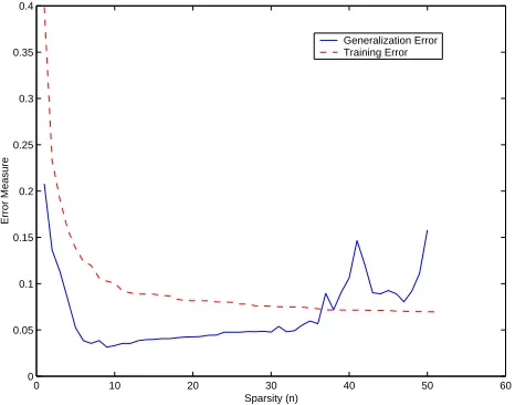
From the description of the greedy algorithms in the previous section, it can be observed that the user is required to specify the required degree of sparsity or an upper bound on the empirical error. Consider the case when no regularization is employed. Then, if the specified degree of sparsity is much higher than the optimal value (or conversely, if the upper bound on the empirical error is smaller than the noise intensity), the model will tend to over-fit the data. To illustrate this phe-nomenon, the typical trends in the generalization error and the training error as a function of the degree of sparsity are shown in Figure 1 for a model problem. It can be clearly seen that there exists an optimum level of sparsity beyond which the model will tend to overfit noise.
0 10 20 30 40 50 60
0 0.05 0.1 0.15 0.2 0.25 0.3 0.35 0.4
Sparsity (n)
Error Measure
Generalization Error Training Error
Figure 1: Trends in the generalization error for a toy dataset when the number of basis functions are increased in the absence of regularization.
It is well known that the problem of overfitting can be overcome by trading-off the empirical risk with model complexity. This observation is embodied in Vapnik’s structural risk minimization principle (Vapnik, 1995). A more traditional approach to this problem employs a regularization parameter to improve generalization. In the present context, we may apply the greedy algorithms to the regularized Gram matrix K+σ2I, whereσ2 is a regularization parameter. Alternatively, a shrinkage parameter (Friedman, 2001) can be used. As a result, the empirical error is guaranteed to converge to a non-zero value. An alternative approach would be to enforce regularization via sparsity, i.e., by finding the optimum level of sparsity which leads to the best generalization perfor-mance. This approach was adopted in Vincent and Bengio (2001), where a validation dataset (or generalized cross-validation) was employed to decide the optimum level of sparsity.
i.e., the one which has the shortest description length. From an information theoretic point of view, this translates into minimizing a code length of the form−log f(
D
|α) +L(α), where f(·|α) represents the data likelihood, given the model parameters (α), while the second term is a measure of the complexity of the model in question. Numerous ways of describing this code length exist in the literature; see Hansen and Yu (2001) for a more detailed exposition of the MDL principle. Of particular interest to us is the two-stage MDL criterion,6 where the model parameters α are selected and L(α)approximated in the first stage. This is followed by a second stage which involves computing the description length of the data, i.e,−log f(D
|α).In the present context of greedily minimizing the L2loss function, applying the two-stage MDL
yields the following approximation to the code length at the l-th stage
m
2 log(r,r) +
l
2log m (10)
Henceforth, the term MDL refers to the two-stage MDL criterion. We compare the MDL cri-terion to the Akaike information cricri-terion (AIC) suitably modified for use in small samples thus (Sugiura, 1978)
m
2 log(r,r) +
l
2
1+l/m
1−(l+2)/m (11)
0 5 10 15 20 25 30 35 40 45 50 0
20 40 60 80 100 120 140
Sparsity (n)
Model Selection Criteria
MDL AIC
Figure 2: The trends of the MDL and AIC criteria for Ripley’s synthetic dataset as a function of the sparsity level.
It can be clearly seen from Equations (10,11) that the first term of both criteria will tend to decrease as more kernels are chosen from the dictionary. In contrast, the second term which repre-sents the model complexity increases at a linear rate. As a consequence when MDL/AIC is used as the termination criterion, the sparsity level for which it reaches a minimum represents an optimal trade-off between empirical risk and model complexity.
In what follows, we use Ripley’s 2D synthetic classification dataset (Ripley, 1996) to show how the MDL and AIC fare as stopping criteria, i.e, by terminating the greedy algorithms when the
minima of MDL/AIC is reached. This data set has 250 training points and 1000 test points and has a Bayes optimal rate of around 8%. Figure 2 shows the trends in the MDL and AIC criteria as the degree of sparsity is increased when a Gaussian kernel with width 0.5 is employed. The decision boundary computed using either of these criteria is shown in Figure 3. Note that for this particular problem, both these criteria yield the same optimum level of sparsity. However, in practice, we have observed that the AIC criterion tends to choose larger models as compared to the MDL criterion. The resulting test errors obtained by employing the sparse model computed using the greedy QR algorithm is 8.8 %, which is close the Bayes optimal rate for this problem. Further, it is interesting to note that the decision boundary in Figure 3 is quite similar to those computed using SVMs and RVMs (Tipping, 2001, pp.222).
−1.5 −1 −0.5 0 0.5 1
−0.2 0 0.2 0.4 0.6 0.8 1 1.2
Figure 3: The centers of the basis functions (circled points) chosen by the MDL criteria for Ripley’s synthetic dataset.
Similar results were obtained for the case of regression using 100 equally spaced samples from a sinc function corrupted with
N
(0,0.1) as training points. It can be seen from Figure 4 that the approximated function using the AIC criterion closely matches the true function using only 8 Gaussian kernels of width 1.0. The root mean square deviation on 1000 equally spaced samples of the true sinc function is 0.0315. Similar conclusions result when the MDL criterion is used to decide the optimum level of sparsity.6. Experimental Investigations
The algorithms presented in this paper were implemented as a library of FORTRAN 77 subroutines which make extensive use of machine optimized BLAS routines. All the numerical experiments reported here were conducted on a single R10000 processor of an SGI Origin 2000 machine with 4.6 Gb main memory. Further note that unlike ORMP, the present algorithms do not require the explicit
a priori computation and storage of the full Gram matrix K. For all experimental investigations,
the elements of the Gram matrix are constructed using a Gaussian kernel of the form k(x1,x2) =
exp(−(x1−x2)2
c ). Unless otherwise stated, the width of the Gaussian kernel c is estimated via a
−10 −8 −6 −4 −2 0 2 4 6 8 10 −0.6
−0.4 −0.2 0 0.2 0.4 0.6 0.8 1 1.2
True Function Estimated Function
Figure 4: The centers of the basis functions (circled dots) chosen by the AIC criteria for approxi-mating the sinc(x) function using 100 noisy samples.
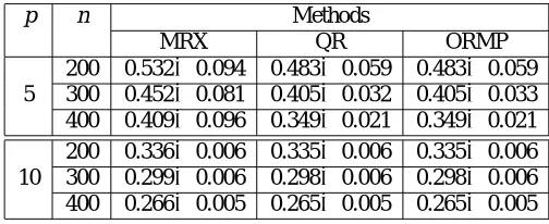
p n Methods
MRX QR ORMP
200 0.532±0.094 0.483±0.059 0.483±0.059 5 300 0.452±0.081 0.405±0.032 0.405±0.033 400 0.409±0.096 0.349±0.021 0.349±0.021
200 0.336±0.006 0.335±0.006 0.335±0.006 10 300 0.299±0.006 0.298±0.006 0.298±0.006 400 0.266±0.005 0.265±0.005 0.265±0.005
Table 1: Comparison of statistics of residuals for 100 realizations of the synthetic datasets generated using F∗.
6.1 Regression Datasets
The algorithms developed in this work are first tested on a synthetic regression dataset generated according to (Friedman, 2001). Subsequently, a detailed comparison study is performed on two real world datasets viz. Boston and Abalone available from the UCI machine learning repository.
We set Gaussian kernel width c to 0.01, 3.9 and 10.0 for the synthetic, Boston and Abalone datasets, respectively. We first generated results by employing the regularized Gram matrix K←
K+σ2I, where σ2 is chosen to be 0.01 for both the synthetic and Boston datasets and 0.1 for Abalone.
The synthetic dataset is generated using a linear combination of 20 basis functions (Friedman, 2001), i.e, F∗(x) =∑20l=1algl(x) +
N
(0,σ2), where x∈Rp and the scalar als are drawn from auniform distribution[0,1]. Here gl(x)= exp{−(x−µl)TΣ−1(x−µl)}, where µl ∈Rpis drawn from
a uniform distribution[0,1]pandΣ∈Rp×pis a randomly generated SPD matrix.
Subset Methods
size (n) MRX QR ORMP
50 14.13±8.07 13.68±7.65 12.17±7.01 100 12.19±7.22 11.19±6.51 10.43±6.47 150 11.08±6.50 10.48±6.01 10.05±7.15 200 8.87±5.67 8.35±5.67 10.13±7.02
Table 2: MSE comparison of MRX, QR & ORMP for the Boston dataset for varying subset sizes.
Subset Methods
size (n) MRX QR ORMP
50 5.04±0.30 4.83±0.29 4.92±0.29 100 4.71±0.19 4.66±0.30 4.66±0.20 150 4.66±0.29 4.65±0.28 4.63±0.25 200 4.52±0.17 4.51±0.27 4.45±0.18 250 4.60±0.25 4.54±0.34 4.57±0.23 300 4.59±0.24 4.55±0.21 4.57±0.25 350 4.68±0.29 4.53±0.29 4.64±0.31
Table 3: MSE Comparison of MRX, QR & ORMP for the Abalone dataset for varying subset sizes.
Table 1 summarizes the results of applying the above techniques to 100 realizations of F∗ for dimensionalities p=5 and p=10, respectively, over a range of subset sizes (n). For each realization, a randomly generated training dataset of 2000 points is used. It appears that the incremental QR and ORMP algorithms are superior to MRX on an average, for either dimensionality (p). However, the differences in performance between the incremental thin QR update technique and ORMP are clearly statistically insignificant.
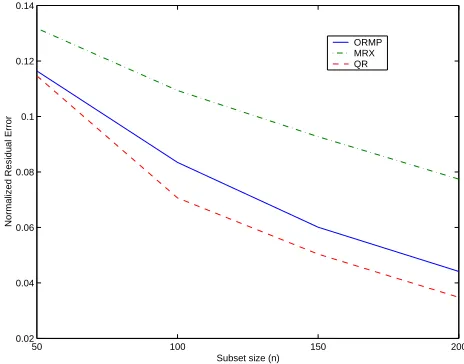
50 100 150 200
0.02 0.04 0.06 0.08 0.1 0.12 0.14
Subset size (n)
Normalized Residual Error
ORMP MRX QR
Figure 5: Convergence of the averaged residual error using greedy algorithms on the Boston dataset.
Dataset QR + MDL QR + AIC Boston 13.3±7.6 (42) 12.9±7.8 (141) Abalone 4.7±0.3 (54) 4.6±0.3 (164)
Table 4: MSE obtained for the Boston dataset when the MDL and AIC criteria are used for com-puting the optimum sparsity level. The average sparsity level is shown in brackets.
of 25 instances. Clearly, the incremental QR factorization update technique succeeds in reducing the residual error the most, while still managing an MSE performance comparable to that of ORMP. This observation along with the attendant computational and storage benefits makes the thin incre-mental QR update technique the algorithm of choice for this dataset. Also note that although MRX loses out in the race for reducing the residual error, its MSE performance is not significantly worse off than ORMP (and QR). For n=200, it actually performs better than ORMP (see Table 2).
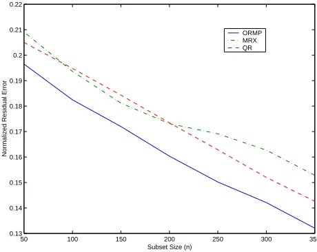
50 100 150 200 250 300 350 0.13
0.14 0.15 0.16 0.17 0.18 0.19 0.2 0.21 0.22
Subset Size (n)
Normalized Residual Error
ORMP MRX QR
Figure 6: Convergence of the averaged residual error using greedy algorithms on the Abalone dataset.
From the results, it can be noted that the best test performance obtained using the greedy thin QR factorization algorithm is 8.3 mean square error with standard deviation 5.7. This is comparable with the best performance achieved by a support vector machine (mean square error 8.7 and standard deviation 6.8) on this dataset; see Table 3 in Sch¨olkopf, Smola, Williamson, and Bartlett (2000). Further, the thin QR algorithm only required around 0.8 seconds to compute the weight vector at the specified sparsity level of 200.
For the Abalone dataset, we averaged our results over 10 random splits of the mother data into 3000 and 1177 training and testing points, respectively. Figure 6 and Table 3 show the convergence trends of the residual error and the mean square testing error, respectively, as the subset size is increased. We observe that the residuals in this case may differ by as much as 13% across the methods considered. In contrast, the corresponding testing errors summarized in Table 3 do not differ significantly.
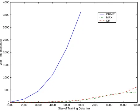
10000 2000 3000 4000 5000 6000 7000 8000 9000 10000 500
1000 1500 2000 2500 3000 3500 4000
Size of Training Data (m)
Wall Time (seconds)
ORMP MRX QR
Figure 7: Comparison of the training time required by various approaches as a function of the size of the training dataset. The subset size (n) is chosen to be 10 % of m.
for the Boston and Abalone datasets. It can be seen from the results that the AIC criterion tends to select larger models as compared to MDL. However, the results for the Boston dataset are not that impressive as compared to those obtained using the regularized Gram matrix. In comparison, both the MDL and AIC criteria worked very well for the Abalone dataset giving test error comparable to that obtained using the regularized Gram matrix. At this point, it is important to point out a de-ficiency in the MRX algorithm: that of slow convergence rate and hence a poor approximation for the residual error when a basis function is added. Since, the MDL and AIC criteria crucially depend on an accurate estimate of the residual, they may fail to predict the optimal trade-off point when used in conjunction with the MRX algorithm. However, this still does not explain the lacklustre performance of the QR algorithm on the Boston dataset. While this feature could well be unique to this dataset, we believe that in practice, a combination of explicit regularization and sparse approx-imation should be effective against most problems.
The final experiment demonstrates the scaling performance of the algorithms presented as the size of the training dataset increases. This study was conducted for the Census dataset (available from the DELVE repository) for the House-Price-8H prototask. Figure 3 shows the computational time as a function of the size of the training dataset for various algorithms. Note that the subset size (n) is set at 10% of the training size. Further note that the timings shown also include the kernel computation time. As expected, the MRX and the greedy thin QR factorization schemes scale impressively when compared to ORMP. In fact, our ORMP simulation seemed to scale worse than what was theoretically expected. We believe this was primarily because our implementation was rich in BLAS Level-1 operations. In contrast, for the MRX and the thin QR algorithm, we could employ Level-2 BLAS routines more extensively.
Methods
Datasets SVM RVM QR + AIC QR + MDL
Error n Error n Error n Error n
Banana 10.9 135 10.8 11 10.7 41 10.9 29
B.Cancer 26.9 117 29.9 6 28.0 11 31.3 5
Diabetes 20.1 109 19.6 4 19.8 4 19.8 4
German 22.6 411 22.2 12 24.8 32 25.6 12
Image 3.0 167 3.9 35 3.1 199 3.5 175
Waveform 10.3 146 10.9 15 12.6 101 11.6 27
Table 5: Comparison of test set percentage errors and sparsity levels for various benchmark classi-fication datasets.
Methods
Digits SVM QR + AIC QR + MDL
Errors n Errors n Errors n
0 16 274 10 699 10 698
1 8 104 9 700 9 695
2 25 377 19 700 19 700
3 19 361 23 699 23 699
4 29 334 25 700 25 697
5 23 388 22 700 22 699
6 14 236 14 699 14 676
7 12 235 11 700 11 699
8 25 342 24 699 24 699
9 16 263 13 700 13 700
Table 6: Comparison of test set errors and sparsity levels for USPS for various methods.
6.2 Classification datasets
Table 5 contrasts the performance and sparsity achieved by the proposed algorithms vis-´a-vis the state-of-the-art Support and Relevance Vector Machines (Tipping, 2001) for a set of benchmark problems.7 While SVMs and RVMs demonstrate comparable generalization behavior, the latter is known to generate models which are often sparser. However, a downside for RVM (and to a lesser extent, the SVM), is the heavy computational cost incurred while training the machine which renders it impractical for large scale data mining. Viewed in this light, Table 5 clearly illustrates the ability of greedy thin QR factorization scheme to generate moderately sparse models (often much sparser than SVMs) while still exhibiting competitive generalization behavior. It is expected that combined with the relatively low training complexity of the thin QR algorithm, this feature would serve well for data mining purposes.
Table 6 compares the generalization performance of the proposed schemes w.r.t. SVMs for the digits in the USPS dataset. The results for SVMs have been taken from Sch¨olkopf et al. (1999). As is common practice for this dataset, the learning task here is that of binary ”one-versus-the-rest” classification for each digit in the database. Note that for most digits, the proposed techniques
generate models which perform at least as well as SVMs, although the training costs incurred in the former are much lower than those in the latter. Further, the increased sparsity levels(n) shown in the table for the proposed techniques are those required by the stopping criteria used. It is important to point out that setting the allowed sparsity level equal to the number of support vectors obtained while training SVMs, results in performance similar to those reported by Vincent and Bengio (2001). Finally, note that in the above experiments, the maximum allowed sparsity level was constrained to 700. Our experiments showed that it is possible to drive the generalization errors further down by increasing this sparsity level. This is corroborated by the trends in the MDL and AIC stopping criteria which (far from rising) continue to decrease even after the sparsity level of 700 is achieved. This behavior of the model selection criteria seems to be a characteristic feature of this dataset.8 However, the accompanying increase in the n may reflect adversely on the runtime complexity of the resulting model.
7. Concluding Remarks
In this paper, we presented greedy learning algorithms for constructing sparse nonlinear regression and classification models using Mercer kernels. An attractive feature of the algorithms presented here is the modest memory requirements and low computational cost incurred. In particular, the computational cost only grows linearly with increase in the size of the training data. This was achieved by exploiting the fact that the use of Mercer kernels leads to an SPD Gram matrix. In particular, this means that the index selection criterion only involves examining the current residual as opposed to working with the normal equations hence saving significantly on the memory re-quirements as well as the computational cost. Together with an effective model selection criterion, the proposed greedy algorithms represent a powerful paradigm for handling both classification and regression problems. This has been amply demonstrated through extensive numerical studies on synthetic as well as real-world benchmark problems.
The empirical studies suggest that the generalization abilities of sparse models constructed using the proposed algorithms for greedy minimization of the L2loss function are competitive with other
state-of-the-art techniques. Since different datasets have widely varying characteristics, it would be difficult to make general statements or predictions about the superiority of one greedy algorithm over the rest. However, if computationally efficiency and memory requirements are a major concern, it appears that the present algorithms are more attractive than existing greedy techniques such as ORMP (Natarajan, 1995), OLS-RBF (Chen, Grant, and Cowan, 1991; Vincent and Bengio, 2001) and L2boost (on Mercer kernels), particularly for large data sets.
It is important to emphasize the absence of tuning parameters (apart from the kernel parameter) in the proposed approach of achieving regularization via sparse approximate interpolation. This property along with the attractive computational benefits make the current approach a promising off-the-shelf tool for machine learning which merits further investigation. An important step towards fulfilling this aim would be developing online versions of the greedy algorithms to improve their computational properties further.
From the point of view of runtime complexity, the present algorithms are generally more at-tractive than SVMs since they typically generate a much sparser solution. However, the converse cannot be ruled out (see, for example, the results for the USPS and Image data). For such cases,
it is natural to consider the possibility of incorporating a sparsity inducing regularizer into the cur-rent framework (Chen, 2001). Alternatively, the relevance vector machine (Tipping, 2001) can be employed to prune the weight vector further.
Acknowledgments
We would like to acknowledge support for this research from BAE Systems - Rolls Royce University Technology Partnership for Design.
References
Adler, J., Rao, B. D. & Kreutz-Delgado, K. (1996). Comparison of basis selection methods.
Pro-ceedings of the 30th Asilomar Conference on Signals, Systems and Computers, Pacific Grove, CA, 1, 252-257.
B ¨uhlmann, P. & Yu, B. (2001). Boosting with the L2 loss: regression and classification. Re-search Report No. 98, Seminar f¨ur Statistik, ETH Z¨urich.
Chen, S. S., Donoho, D. L. & Saunders, M. A. (1998). Atomic decomposition by basis pursuit.
SIAM Journal on Scientific Computing, 20, 33-61.
Chen, S., Cowan, C. F. N., & Grant, P. M. (1991). Orthogonal least squares learning for radial basis function networks. IEEE Transactions on Neural Networks, 2(2), 302–309.
Chen, S., (2001) Local regularization assisted orthogonal least squares regression. IEEE
Trans-actions on Neural Networks, submitted.
Chow, E., & Saad, Y. (1997). Approximate inverse techniques for block-partitioned matrices.
SIAM Journal of Scientific and Statistical Computing, 18(6), 1657-1675.
Chow, E., & Saad, Y. (1998). Approximate inverse preconditioners via sparse-sparse iterations.
SIAM Journal of Scientific and Statistical Computing, 19(3), 955-1023.
Couvreur, C., & Bresler, Y. (1999). On the optimality of the backward greedy algorithm for the subset selection problem. SIAM Journal on Matrix Analysis and Its Applications, 21 (3), 797-808.
Daniel, J. W., Gragg, W. B., Kaufmann, L., & Stewart, G. W. (1976). Reorthogonalization and stable algorithms for updating the Gram Schmidt QR factorization. Mathematics of Computation,
30 (136), 772-795.
Evgeniou, T., Pontil M., & Poggio T. (2000). Regularization networks and support vector ma-chines. Advances in Computational Mathematics, 13, 1-50.
Freund, Y. & Schapire, R. E. (1996). Experiments with a new boosting algorithm. Proceedings
of the 13th International Conference on Machine Learning. Morgan Kauffman, San Francisco,
148-156.
Friedman, J. H. (2001). Greedy function approximation: a gradient boosting machine. Annals
of Statistics, 29 (5), 1189–1232.
Friedman, J. H., Hastie, T. & Tibshirani, R. (2000). Additive logistic regression: a statistical view of boosting. Annals of Statistics, 28, 337-407 (with discussion).
Girosi, F. (1998). An equivalence between sparse approximation and support vector machines.
Neural Computation, 10, 1455-1480.
Grote, M. J. & Huckle, T. (1997). Parallel preconditioning with sparse approximate inverses.
Hansen M. H. & Yu, B. (2001). Model selection and the principle of minimum description length. Journal of the American Statistical Association, 96(454), 746-774.
Judd, K. & Mees, A. (1995). On selecting models for nonlinear time-series. Physica D, 82(4), 426-444.
Mallat, S. & Zhang, Z. (1993). Matching pursuit in a time-frequency dictionary. IEEE
Trans-actions on Signal Processing, 41, 3397–3415.
Natarajan, B. K. (1995). Sparse approximate solutions to linear systems. SIAM Journal of
Computing, 25(2), 227-234.
Natarajan, B. K. (1999). On learning functions from noise-free and noisy examples via Occam’s razor. SIAM Journal of Computing, 29(3), 712-727.
Reichel, L., & Gragg, W. B. (1990). Algorithm 686: FORTRAN Subroutines for Updating the QR Decomposition. ACM Transactions on Mathematical Software, 16 (4), 369-377.
Ripley, B. D. (1996). Pattern Recognition and Neural Networks. Cambridge University Press. Schaback, R., & Wendland, H. (2000). Adaptive greedy techniques for approximate solution of large RBF systems. Numerical Algorithms, 24(3), 239-254.
Sch¨olkopf, B., Sung, K., Burges, C., Girosi, F., Niyogi, P., Poggio, T. & V. Vapnik. (1997). Comparing support vector machines with Gaussian kernels to radial basis function classifiers. IEEE
Transactions on Signal Processing, 45, 2758 - 2765.
Sch¨olkopf, B., Smola, A. J., Williamson, R., & Bartlett, P. (2000). New support vector algo-rithms. Neural Computation, 12(5), 1207-1245.
Smola, A. J., & Bartlett, P. L. (2001). Sparse greedy Gaussian process regression. Advances in
Neural Information Processing Systems 13, MIT Press, 619-625.
Smola, A. J., & Sch¨olkopf, B. (2000). Sparse greedy matrix approximation for machine learn-ing. Proceedings of the 17th International Conference on Machine Learning, Morgan Kaufmann, 911-918.
Sugiura, N. (1978). Further analysis of the data by Akaike’s information criterion and the finite corrections. Communications in Statistics, A7, 13-26.
Tipping, M. E. (2001). Sparse Bayesian learning and the relevance vector machine. Journal of
Machine Learning Research, 1, 211-244.
Vapnik, V. (1995). The nature of statistical learning. New York: Springer Verlag.
Vincent, P., & Bengio, Y. (2001). Kernel Matching Pursuit. Machine Learning, 48 (1-3), 165-187.
Williams, C., & Seeger, M. (2001). Using the Nystr¨om method to speed up kernel machines.
Advances in Neural Information Processing Systems 13, MIT Press, 682-688.
Zhang, T., (2001). Some sparse approximation bounds for regression problems. Proceedings of