Impact of Seismic Vulnerability on Bridge Management Systems

(1)

IMPACT OF SEISMIC VULNERABILITY ON BRIDGE MANAGEMENT SYSTEMS

IMP

ACT

OF

SEI

SMIC

VUL

NER

ABI

LI

T

Y

ON

BRIDGE

MAN

AGEMEN

T

SY

ST

EMS

M

a

y

2

0

1

2

Y

ANC

HAO

Y

UE

(2)

University of Trento

University of Brescia

University of Padua

University of Trieste

University of Udine

University IUAV of Venice

Yanchao Yue

IMPACT OF SEISMIC VULNERABILITY

ON BRIDGE MANAGEMENT SYSTEMS

Tutor: Dr. Daniele Zonta

Co-Tutor: Dr. Matteo Pozzi

(3)

Impact of Seismic Vulnerability on Bridge Management Systems

UNIVERSITY OF TRENTO

Doctoral School of Engineering of Civil and Mechanical Structural Systems

Head of Doctoral School: Prof. Davide Bigoni

Dissertation Defense on 25th November 2011

Board of Examiners:

Prof. Paolo E. Pinto University of Rome 'La Sapienza', Italy

Prof. Daniel Straub Technical University of Munich, Germany

(4)

SUMMARY

Motivated by the potential vulnerability of their road infrastructure, many national authorities and local Departments of Transportation are incorporating seismic risk assessment in their management systems. This Dissertation aims to develop methods and tools for seismic risk analysis that can be used in a Bridge Management System (BMS); helping bridge owners to assess the costs of repair, retrofit and replacement of the bridges under their responsibility.

More specifically, these tools are designed to offer estimates of:

(1) the seismic risk to single components of bridges and their expected performance after an earthquake.

(2) the impact a priori (i.e. before an earthquake) of a given earthquake on the

operation of a road network, in terms of connectivity between different locations.

(3) the damage a posteriori (i.e. after an earthquake) to road network operation,

based on prior knowledge of network vulnerability and on the observed damage to a small number of single bridges.

The effectiveness of these methods is tested and validated in a specific case study, the bridge stock of the Autonomous Province of Trento (APT) in Italy.

To address the first point, I will first introduce the fragility curve method for risk assessment of individual bridges. The Hazus model is chosen as the most appropriate and is applied to the bridges of the APT stock. Once the fragility curves for all the bridges have been generated, a risk analysis is performed for three earthquake scenarios (with return periods of 72, 475 and 2475 years) and four condition states (operational, damage, life safety and collapse limit state). Next, I will extend the results of the component level analysis to the network level: the APT road network is modeled in the form of a graph and the problem of connectivity between two locations is analyzed. A shortest path algorithm is introduced and implemented to identify the best path between any two given places. Correlation in capacity and demand among bridges is not considered at this stage.

(5)

(6)

DEDICATION

To my parents, my wife and Elena:

(7)

(8)

ACKNOWLEDGEMENTS

My first and utmost gratitude is to my tutor, Dr. Daniele Zonta for his invaluable supervision and support during my PhD study. His profound knowledge of the research field and his manner of viewing this world have always inspired me, not only in the way of conducting my research work but also in the way of striving in my life. His generous encouragements and great enthusiasm in my job have and will always stimulate me to face challenges with confidence, all my life. I am lucky to have the honor of being his student in my life.

I wish to express my special thanks to Dr. Matteo Pozzi and Dr. Francesca Bortot. The extensive discussions and close cooperation with them resulted in many of the innovative ideas presented in this Thesis. Especially, I need to thank my co-tutor Dr. Matteo Pozzi, who reviewed and checked every detail of my Thesis.

My thanks also go to Prof. Riccardo Zandonini, Prof. Maurizio Piazza and Prof. Oreste S. Bursi for their instructions and support in Trento and to my friends and colleagues, Huayong Wu, Chuanguo Jia, Davide Trapani, Emiliano Debiasi, Federico Larcher, Paolo Esposito, Anil Kumar, Leqia He, and Zhen Wang, who made my stay here feel as if it were my home.

(9)

(10)

LIST OF TABLES

Table 1.1 Deadliest Earthquakes 1990 - 2011 (USGS, 2011) ... 20

Table 2.1 Definition of damage states (FEMA, 2003) ... 31

Table 2.2 Drift and displacement limits (Basöz and Mander, 1999) ... 32

Table 2.3 Values for strength reduction factor Q (Dutta, 1999) ... 33

Table 2.4 Friction coefficients of the bearings in the transverse direction (Basöz and Mander 1999) ... 34

Table 2.5 3D effect factor for bridges seated on strong bearings with weak piers (Dutta and Mander 1998) ... 35

Table 2.6 3D effect factor for single span bridge (Basöz and Mander 1999) ... 35

Table 2.7 The required parameters for calculating median spectral accelerations .... 36

Table 2.8 Seismic probability of Ponte Nogarè SP83 for different limit states ... 37

Table 2.9 Spectral parameters at the SP90 Adige Bridge location ... 38

Table 2.10 parameters of the SP90 Bridge on the Adige River ... 38

Table 2.11 parameters of the pier ... 39

Table 3.1 probabilities in operational mode... 50

Table 3.2 all the network states in Fig. 3.1 ... 51

Table 3.3 Geographical coordinates of nodes in Trento to Ala road network ... 55

Table 3.4 Descriptions of links in Trento to Ala road network ... 57

Table 3.5 Expected connectivity of between Trento to Ala given different m values ... 60

Table 3.6 Connectivity between Passo Lavazè and Riccomassimo for different m values for return period of 475 years ... 61

Table 3.7 Connectivity between Passo Lavazè and Riccomassimo for different m values for return period of 72 years ... 62

Table 3.8 Connectivity between Passo Lavazè and Riccomassimo given different m values for return period of 2475 years ... 62

Table 4.1 States of the variables (Neapolitan, R.E. 2003) ... 75

Table 4.2 List of all the software package for BNs ... 90

(15)

Table 5.3 Results given the evidence ... 118

Table 5.4 Parameters for calculating median spectral acceleration ... 119

Table 5.5 Prior distribution of variables after initialization ... 120

Table 5.6 Posterior distributions of variables given the evidence ... 121

Table 5.7 Posterior distributions of the physical parameters given the evidence .... 121

Table 6.1 Prior distribution of the global variables ... 131

Table 6.2 Posterior distributions of the global variables based on the evidence that bridge 1 has collapsed ... 134

Table 6.3 Posterior distributions of the global variables based on evidence that bridge 2 has collapsed ... 135

(16)

LIST OF FIGURES

Fig. 1.1 Bridge age distribution (a); typological distribution (b) in APT-BMS (Zonta.

et al 2007) ... 22

Fig. 1.2 Flowchart for the APT-BMS showing its main components and information paths (Zonta. et al 2007) ... 22

Fig. 2.1 Graphical representation of fragility function (Nielson 2005) ... 28

Fig. 2.2 Two failure modes for single span bridges (Basöz, and Mander. 1999) ... 33

Fig. 2.3 (a) Overview of the SP83 Bridge on the Nogarè River; (b) Plan view, elevation and cross-section of the deck ... 36

Fig. 2.4 Fragility curves of Ponte Nogarè SP83 ... 37

Fig. 2.5 Overview of the SP90 Bridge on the Adige River at Villa Lagarina ... 37

Fig. 2.6 The fragility curves of the pier ... 38

Fig. 2.7 The fragility curves due to the sliding of bearings ... 39

Fig. 2.8 Seismic vulnerability of APT stock for the return period of 475 years in damage states (a), OLS (b), DLS (c), LLS (d), CLS ... 40

Fig. 2.11 Seismic vulnerability distribution of the APT stock ... 42

Fig. 2.12 PGA value of APT region with 475 years’ return period (DPC-INGV) ... 42

Fig. 2.13 Example of empirical fragility curves reported by Shinozuka et al. (2000b) ... 44

Fig. 3.1 Simple network with two nodes and three bridges ... 50

Fig. 3.2 Google Earth map from Trento to Ala ... 55

Fig. 3.3 Simulated transportation graph between Trento-Ala ... 56

Fig. 3.4 The simplified graph between Trento-Ala ... 56

Fig. 3.5 Google Earth map of the APT-BMS network ... 58

(17)

probability of link failure ... 59

Fig. 3.8 Locations of Passo Lavazè and Riccomassimo in APT road network ... 61

Fig. 3.9 Calculation procedures of a simple graph using Dijkstra’s algorithm ... 64

Fig. 3.10 Simulated network and the safest path between Passo Lavazè and Riccomassimo ... 65

Fig. 4.1 A Bayesian Network for the example in Section 4.2.4 ... 77

Fig. 4.2 Junction tree structure for the Bayesian Network in Fig 4.1 ... 78

Fig. 4.3 Moralization procedures for the Bayesian Network in Fig 4.1 ... 79

Fig. 4.4 Triangulation procedures for the Bayesian Network in Fig 4.3 ... 79

Fig. 4.5 A conditional Gaussian BN ... 81

Fig. 4.6 Graphical representation of the direct combination of two potentials ... 83

Fig. 4.7 Example of Bayesian Network ... 86

Fig. 4.8 Assignments of the potentials to the cliques ... 86

Fig. 4.9 The order of collecting messages ... 87

Fig. 4.10 Order of distributing messages ... 88

Fig. 4. 11 Example of graph structure ... 90

Fig. 4.12 Graphical representation of the ‘Sick Dilemma’ example in Hugin ... 92

Fig. 4.13 Prior distribution of the ‘Sick Dilemma’ example after initialization in Hugin ... 92

Fig. 4.14 Graphical representation of the ‘Sick Dilemma’ example in BayesiaLab . 93 Fig. 4.15 Node editor in BayesiaLab ... 93

Fig. 4.16 Software window of Netica ... 94

Fig. 4.17 The software window of MSBNX ... 94

Fig. 5.1 Conceptual framework of BN in Bensi et al. (2010) ... 100

Fig. 5.2 The conceptual BN that contains the three main parts in the framework .. 101

Fig. 5.3 The closest distance to the surface projection of the fault (Bensi, 2010) ... 104

Fig. 5.4 Bayesian Network for bridge type 1... 108

Fig. 5.5 Bayesian Network for bridge type 2... 108

Fig. 5.6 Bayesian Network for two bridges with strong piers and weak bearings .. 110

Fig. 5.7 Bayesian Network for two bridges with strong bearings and weak piers .. 111

Fig. 5.8 5-component MoG Approximation of the truncated exponential distribution ... 113

Fig. 5.9 CDFs of the truncated exponential distribution and MoG Approximation 113 Fig. 5.10 How to incorporate into the framework the evidence about the bridge state ... 114

Fig. 5.11 Procedures to generate the random number X1 ... 114

Fig. 5.12 SP135 Bridge on River Fersina-Canezza (a) overview (b) Plan view, elevation and cross-section of the deck ... 116

Fig. 5.13 SP31 Bridge on River Avisio (a) overview (b) Plan view, elevation and cross-section of the deck ... 117

(18)

Fig. 5.15 Viadotto San Silvestro(a) overview (b) plan view, elevation and

cross-section of deck ... 119

Fig. 6.1 The BN framework for the network with n bridges ... 125

Fig. 6.2 BN model for intra-event error (Bensi, 2010) ... 126

Fig 6.3 Line layout, circle layout and grid layout for numerical investigation (Bensi, 2010) ... 127

Fig. 6.4 Error measures for different configurations at different distances based on the methods in Bensi (2010) ... 128

Fig. 6.5 The BN framework for a network with n bridges ... 129

Fig. 6.6 Distance between two bridges A and B at different locations. ... 132

Fig. 6.7 Prior seismic vulnerability in APT bridge stock for a 7.0 magnitude earthquake with epicenter in Salò (E10.519935,N45.603110.) ... 133

Fig. 6.8 Prior distribution of probability of collapse in APT bridge stock for a 7.0 magnitude earthquake with epicenter in Salò (E10.519935,N45.603110) ... 134

Fig. 6.9 Posterior seismic vulnerability in APT bridge stock for a 7.0 magnitude earthquake with the epicenter in Salò (E 10.519935,N 45.60311) ... 136

Fig. 6.10 Posterior distribution of probability of collapse in APT bridge stock for a 7.0 magnitude earthquake with the epicenter in Salò (E10.519935, N45.603110) . 136 Fig. 6.11 Link composed by bridge A and bridge B in series ... 137

Fig. 6.12 Link formed by n bridges in series ... 138

Fig. 6.13 Different links between two nodes ... 139

Fig. 6.14 The network between Trento and Ala ... 141

Fig. 6.15 The link between node 2 and node 4 ... 141

Fig. 6.16 The BN used to calculate the value of P(B425|B424) ... 142

Fig. 6.17 The BN used to calculate the value of P(B426|B425∙B424) ... 143

Fig. 6.19 The best path between Passo Lavazè and Riccomassimo ... 144

(19)

(20)

1 Introduction

1.1 Motivation

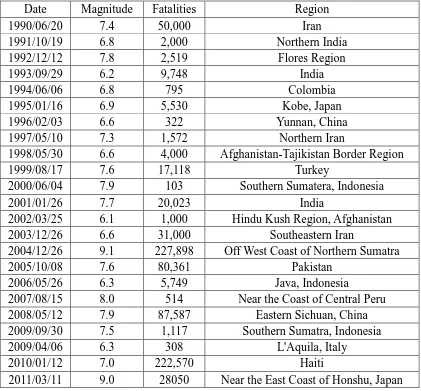
The recent Magnitude 9.0 earthquake near the East Coast of Honshu, Japan, causing 28050 deaths (USGS 2011), again heightens our awareness of the great damage that can be caused by earthquakes. There are about five million earthquakes per year, worldwide. They can cause fires, floods, toxic gas leaks, the spread of bacteria and radio-active materials and can also cause tsunamis, landslides, avalanches, cracks and other secondary disasters. Table 1.1, taken from USGS (2011), gives a quantitative idea of how enormous the damage produced by earthquakes to human society in the last twenty years has been.

Bridges, in particular, play a vital role in modern transportation: they are the key nodes of various road networks and the main components of three-dimensional city traffic. Bridges are also the reflection of a country's development, economic strength, technology and productivity. Bridge Management Systems (BMS) are tools designed to help bridge managers keep track of their bridge stock: providing information on the bridge stock characteristics, condition and serviceability (Thompson et al. 1998, Astudillo 2002, Frangopol Neves 2004, and Bortot 2006). Based on the analysis of single bridges, the BMS helps bridge managers develop programs to determine the best allocation of resources to maximize the safety and functionality of the road network. Originally, the function of BMS was to facilitate the day-to-day management of bridges. Gradually, the functions of BMS became more and more powerful (Bortot 2006). More recently, bridge management systems have been used as tools to improve the overall condition of bridges and to prevent excessive structure deterioration (Bortot, 2006).

(21)

example of the 1995 Kobe Earthquake, when at least 60% of the bridges in the Kobe area were damaged and the Hanshin Expressway, the major transportation route between Osaka and Kobe, collapsed.

Motivated by the potential vulnerability of their road infrastructure, many national authorities and local Departments of Transportation are incorporating seismic risk assessment in their management systems (FEMA 2003, Shinozuka et al. 2000). Therefore, there is growing demand for tools that help assess seismic bridge vulnerability and can predict bridge performance under a given earthquake scenario. Of critical importance to strategic decision making by transportation and civil protection agencies, is the ability to predict the operational state of the road network in a post-earthquake scenario; this can help minimize the impact of possible network downtimes on the rescue operations.

Table 1.1 Deadliest Earthquakes 1990 - 2011 (USGS, 2011)

Date Magnitude Fatalities Region

1990/06/20 7.4 50,000 Iran

1991/10/19 6.8 2,000 Northern India

1992/12/12 7.8 2,519 Flores Region

1993/09/29 6.2 9,748 India

1994/06/06 6.8 795 Colombia

1995/01/16 6.9 5,530 Kobe, Japan

1996/02/03 6.6 322 Yunnan, China

1997/05/10 7.3 1,572 Northern Iran

1998/05/30 6.6 4,000 Afghanistan-Tajikistan Border Region

1999/08/17 7.6 17,118 Turkey

2000/06/04 7.9 103 Southern Sumatera, Indonesia

2001/01/26 7.7 20,023 India

2002/03/25 6.1 1,000 Hindu Kush Region, Afghanistan

2003/12/26 6.6 31,000 Southeastern Iran

2004/12/26 9.1 227,898 Off West Coast of Northern Sumatra

2005/10/08 7.6 80,361 Pakistan

2006/05/26 6.3 5,749 Java, Indonesia

2007/08/15 8.0 514 Near the Coast of Central Peru

2008/05/12 7.9 87,587 Eastern Sichuan, China

2009/09/30 7.5 1,117 Southern Sumatra, Indonesia

2009/04/06 6.3 308 L'Aquila, Italy

2010/01/12 7.0 222,570 Haiti

(22)

1.2 Objectives of the Thesis

This Dissertation aims to develop methods for seismic risk analysis that can be incorporated in a BMS and so help bridge owners to assess the costs of repair, retrofit and replacement of the bridges under their responsibility. More specifically, these tools address the following points:

1. Estimating the seismic risk of the individual components of a bridge stock,

and their expected performance after an earthquake.

2. Evaluating a priori (i.e. before an earthquake) the impact of a given

earthquake on the operation of a road network, in terms of connectivity between different locations.

3. Evaluating a posteriori (i.e. after an earthquake) the damage state of a road

network and its operability, based on the prior knowledge of the network vulnerability and the posterior evidence of damage observed on one or more individual bridges.

The effectiveness of these tools is tested and validated on a specific case study, the bridge stock of the Autonomous Province of Trento (APT) in Italy. The APT bridge stock and the Bridge Management Systems currently used by the Department of Transportation are briefly introduced in the next Section.

1.3 Introducing the APT BMS

(23)

Impact of Seismic Vulnerability on Bridge Management Systems a) 0 20 40 60 80 100 120 140 160 180 200

1905 1915 1925 1935 1945 1955 1965 1975 1985 1995 2005 year of construction

n u m b e r o f b ri d g e s b) prestressed concrete 32.41% steel and steel concrete composite 8.23% reinforced concrete 30.53% reinforced concrete and steel arch 4.46% unreinforced concrete and mansory arch 24.38%

Fig. 1.1 Bridge age distribution (a); typological distribution (b) in APT-BMS (Zonta. et al 2007) COMMON STATE CS INVENTORY INSPECTION SYSTEM PR.IS.02 PR.IS.03 PR.IS.04 PR.IS.05 RELIABILITY  BRIDGE STOCK APT Dot ARCHIVE OTHER SOURCES inspector evaluator DETERIORATION MODEL TIME-VARIANT RELIABILITY MODEL COST MODEL INSPECTION SYSTEM PR.IS.01 P ROCE DUR E S ASSESSMENT SYSTEM PR.VS.01 PR.VS.02 PR.VS.03 PR.VS.04 PR.VS.05 NETWORK LEVEL DATA MAINTENANCE MODEL External experts BMS manager @ SOS PAT DECISION-MAKING TOOLS DB M O DE L S BMS update group @ UniTN inspector P E O P L E

(24)

The APT-BMS has been operational since 2004; it manages 986 bridges and approximately 2400 kilometers of roads. Most of the APT bridges were built after the Second World War; the peak construction period being the 70s (Fig. 1.1(a)). As for construction type (Fig. 1.1(b)), 62.93% of APT bridges are reinforced concrete and prestressed concrete, and 28.84% are arch bridges, while the remaining 8.23% includes steel and steel-concrete composite bridges.

The APT-BMS is based on an SQL database, which includes all the data for the whole stock of bridges. The main characteristics of the systems are:

 The system is fully operative on the web; inspectors and evaluators upload data

to the system through a web-based interface and the managers access the results of the analysis using the same web interface.

 All personnel including DoT (Department of Transportation) managers, DoT

inspectors and professional engineers involved in management can directly interact with the system.

 All information is provided in real-time.

 For each bridge, the system not only gives a clear indication of the condition

state but also its safety level expressed as a reliability index.

 System maintenance and upgrade are continuous and transparent to the users.

As shown in Fig. 1.2, the APT-BMS has four major components: ‘Data Storage’, ‘Maintenance and Cost Model’, ‘Deterioration Model’ and ‘Decision Making Algorithms’. These components are divided into modules; each module having a specific task. The module can be at project level or network level. The former focuses on a single bridge while the latter concerns the bridge stock as a whole.

(25)

1.4 Method

Objective 1 is addressed using a classical fragility curve approach. Fragility curves are conditional probability statements which give the likelihood of a bridge reaching, or exceeding, a particular damage level for an earthquake of a given intensity level (Shinozuka et al. 2000a, Nielson 2005). Much research has been devoted to generating fragility curves. Because of the characteristics of APT-BMS, managing a large number and variety of bridge types, a systematic and quick method is required to develop fragility curves. The Hazus model (FEMA, 2003) meets this requirement and was chosen for application to the case study: in contrast with other methods, such as empirical fragility curves or analytical fragility curves that require much previous damage data or extensive computation, only limited information is needed for this model. Using the Hazus model, the fragility curves for all the bridges in the APT stock are generated. Next, the seismic risks for a number of earthquake scenarios are evaluated. I considered 3 earthquake scenarios, with return periods of 72, 475 and 2475 years, and four possible limit states of the bridge: operational (OLS), damage (DLS), life safety(LLS) and collapse (CLS).

After an earthquake, the ability to decide the best path to distribute the available human and material rescue resources to the disaster centre is of paramount

importance to decision makers. Addressing Objective 2 means solving the problem

of determining the best path between any two given locations after an earthquake, where ‘best’ means the lowest risk of exposure to operational problems in a given damage scenario. This problem is addressed by Dijkstra’s algorithm (Dijkstra, 1959). In the analysis, bridges are first regarded simply as independent components. Next, their mutual correlation in demand and capacity are taken in to account. For example, nearby bridges are likely to have a similar site condition, thus their seismic demands are somehow correlated. Also, some of the bridges have very similar characteristics, such as type, material, and construction year. In this case, it is reasonable to find the correlations between these bridges and so provide a dynamic assessment of seismic risk.

To address Objective 3, I propose to model the logical connection between the

(26)

individual bridges and the prior probabilities of the bridge being in any one of the limit states are calculated during the initialization procedures. After an earthquake, the data on the bridge is entered into the network using the Monte-Carlo method and the probabilities of other variables are updated. Next, this framework is easily extended from individual bridges to the whole network; all the bridges in the network are correlated through the demand model and the capacity model. When an earthquake happens, the data on one or more of the bridges can be propagated throughout the network, so as to provide an updated assessment on the performance of the other bridges and the whole network. Finally, the best path search between any two given network nodes is reformulated, now accounting for bridge correlations in demand and capacity.

1.5 Outline of Thesis

The rest of the Thesis is organized in the following Chapters, in detail:

 In Chapter 2, the fragility curve method for risk assessment is introduced. The

Hazus model is chosen as the most appropriate and is applied to the bridges of the APT stock. Once the fragility curves for all the bridges have been generated, risk analysis is performed for three earthquake scenarios (with return periods of 72, 475 and 2475 years) and four damage states (OLS, DLS, LLS, and CLS).

 In Chapter 3, I extend the results of the component analysis to the network level;

the APT road network is modeled in the form of a graph and the problem of connectivity between two locations is analyzed. A shortest path algorithm is introduced and implemented, to identify the best path between any two given places. Correlation in capacity and demand among bridges is not accounted for at this stage.

 Chapter 4 describes basic Bayesian Networks theory. After reiterating the

fundamentals of probability theory, the definition of the Bayesian Network is given. The general operations on Bayesian Networks are introduced and the computation scheme with conditional Gaussian distributions is explained in detail.

 Chapter 5 presents a seismic risk assessment framework both for individual

(27)

 In Chapter 6, the concept introduced in Chapter 5 for two bridges is extended to

all the bridges in the network of the post-earthquake assessment system. Now, all the bridges are correlated through the demand model and capacity model. Given the data on one or more variables, the performance of the whole network can be updated. The best path given any two nodes within the network is identified again. Correlations between different bridges are now considered and the results are compared with those in Chapter 3.

 Finally, in Chapter 7, the outcomes and limits of this Thesis are summarized and

(28)

2 Fragility curves

2.1 Introduction

Fragility curves are conditional probability statements which give the likelihood of a bridge reaching, or exceeding, a particular damage level, for an earthquake of a given intensity level (Shinozuka et al. 2000a, Nielson 2005). The conditional probability is given by the following equation:

) |

( ) (

Fragility x P LS IM x _(2.1)

where LS is the limit state of the bridge, IM is the ground motion intensity measure of the bridge, and x is the realization of the intensity measure. This equation shows that when the earthquake intensity is x, the probability of the bridge exceeding the

limit state LS is Fragility(x). Fig. 2.1 is the graphical representation of Equation

(2.1).

As an effective tool in seismic risk analysis, fragility curves have become more and more popular. Fragility curves are not only useful in seismic risk assessment, but also in bridge retrofit prioritization and post earthquake response. When updating a bridge network, fragility curves can be used to highlight the most vulnerable bridges so as to maximize the functionality of the whole bridge network system. In a real time post earthquake situation, fragility curves can assist decision makers to make rapid decisions on bridge closures.

(29)

P LS

x

P(LS

|IM=

x

)

1.00

0.00

IM P

LS

x

P(LS

|IM=

x

)

1.00

0.00

IM

Fig. 2.1 Graphical representation of fragility function (Nielson 2005)

2.1.1 Expert Based Fragility Functions

One example of Expert-based Fragility Functions is ATC-13 (ATC, 1985), developed by the Applied Technology Council (ATC) and reported by Nielsen (2005). The ATC put together 42 experts to give information on the various components of infrastructures. The experts were asked to give the probability of a bridge being in one of seven damage states for a given intensity value. These results were compiled as the damage probability matrices (DPM) for bridges in the ATC-13 report (ATC, 1985). Nielsen (2005) raised several major concerns with this methodology: first, the procedure is subjective in that it is based solely on the experience of the experts; next, the DPM were created for only two classes of bridges, major and conventional. He concluded that this method presents a very high level of uncertainty. See Nielsen (2005) for more details.

2.1.2 Empirical fragility curves

(30)

Although the generation methods for empirical fragility curves are relatively straightforward, they have some drawbacks and limitations as pointed out by Basöz and Kiremidjian (1995). First, it is difficult to get enough information on bridges belonging to a specific bridge class that lie in a particular damage level. Second, it is very difficult to get the ground motion intensities for the target bridges. Finally, the empirical fragility curves are too subjective. There is often a discrepancy between the damage levels assigned by two different inspectors. Further details of this discussion are found in Basöz and Kiremidjian (1995).

2.1.3 Analytical fragility curves

Because of the limitations of empirical fragility curves, more research is devoted to the implementation of analytical fragility curves. When actual bridge damage and ground motion data are not available, analytical fragility curves must be used to assess the performance of bridges under earthquakes. There are many researchers who have developed analytical fragility curves for bridges using a variety of different methodologies.

According to the definition of the fragility curves (Shinozuka et al. 2000a, Nielson 2005), it is obvious that fragility curves are related to both structural demand (D) and structural capacity (C). The fragility can be described as:

] 0 ln [ln ]

[    

 P D C P D C

P_f (2.2)

In addition, when the structural demand and capacity fit a lognormal distribution - if we assume that: C  lnN (C, C2); D  lnN (D, D2), then the reliability index 

is:

P P    

 (2.3)

where P = D - C, P2 = C2 + D2.

(31)

2.2 HAZUS model

HAZUS (FEMA 2003) is a geographic information system (GIS) based, standardized, nationally applicable multi-hazard loss estimate methodology and software that was developed for the National Institute of Building Science (NIBS) under a cooperative agreement with the Federal Emergency Management Agency (FEMA). Hazus is intended to develop guidelines and procedures for making earthquake loss estimates. It can be used by local, state and regional officials to help them to reduce risks from earthquakes, and to prepare for emergency response and recovery. This package was developed by a team of earthquake loss experts including earth scientists, engineers, architects, economists, emergency planners, social scientists and software developers. It provides damage and loss estimate for thirteen major components or subcomponents, for example general building stock, transportation systems, airport transportation systems, and so on.

The HAZUS model (FEMA, 2003) is a rapid approach seeking to establish dependable fragility curves (Mander, 1999). In contrast to other methods that have been used in the past, such as empirical fragility curves or analytical fragility curves that require much previous damage data or extensive computation, only limited information is needed for this model.

Because of the characteristics of the APT bridge stock, illustrated in Section 1.2, with a large number and variety of bridge types, a systematic and quick method is required to develop fragility curves. Given the level of information stored in the APT-BMS database, HAZUS seems the most suitable model for this application. Its implementation in the APT-BMS is explained in here.

2.2.1 Formulation of fragility curves

The probability of being in or exceeding a damage state in HAZUS is modeled as:

1

[

(

)]

Φ[ ln(

)]

Α

(

)

a f a i

g i

S

P S

a

=

i=1, 2 , 3, 4 (2.4)

where is the standard normal cumulative distribution function; Sa is the spectral

acceleration amplitude (for a period of T=1 sec); (ag)i is the median spectral

acceleration that causes the ith damage level; and is the normalized composite

log-normal standard deviation. There are five possible damage states defined in APT-BMS: no-damage, OLS, DLS, LLS, and CLS; these five states are associated with the five damage state defined in Hazus according to Table 2.1. The normalized

(32)

and demand. As justified by Basöz and Mander (1999), the uncertainty factor for seismic demand can be assumed to be 0.5 (Pekcan, 1998), the uncertainty factor for capacity is assumed to be 0.25 (Dutta, 1999), and an analysis uncertainty factor is

assumed to be 0.2. Therefore the recommended value of =(0.52+0.252+0.22)0.5 =

0.6. Therefore, in Equation (2.4), the only unknown parameter is (ag)i, which can be

calculated using a capacity-spectrum approach.

Table 2.1 Definition of damage states (FEMA, 2003)

Damage state Failure Mechanisms

1 No damage First yield

2 Operational limit state (OLS) Cracking, spalling

3 Damage control limit state (DLS) Bond, abutment back wall

collapse

4 Life safety limit state (LLS) Pier concrete failure

5 Collapse limit state (CLS) Deck unseating, pier collapse

2.2.2 Capacity-spectrum approach

According to the Italian code (D.M.14 Jan 2008), which is largely based on Eurocode 8 (Eurocode 8, 2004), the seismic demand is given by:

0

(C_d)_S a_g  S η F (2.5a)

0

( ) C

d L g

T

C a S η F

T  

 _{     }

  (2.5b)

where (Cd)S, (Cd)L are the seismic demands of short and long periods; ag is the design

ground acceleration (normalized with respect to gravitational acceleration,g); S is

the coefficient dependent on the soil type; is the damping correction factor with a

reference value of for 5% viscous damping; F0 is the spectral amplification

factor; TCis the upper limit of the period of the constant spectral acceleration branch;

and T is the effective period of the structure given by:

Δ Δ

2 2 2

y c

W W

T π π π

g k g F C g



     

(33)

where W is the weight of the bridge; Fy is the lateral force on the pier; Cc= Fy / W is

the base shear capacity; and is maximum displacement response. For example, for

a collapse mechanism involving bridge pier bending collapse, the ultimate displacement can be calculated using:

Δ θ H (2.7)

where is the column drift, and H is the column height (Basöz and Mander 1999).

Basöz and Mander (1999) also propose values of  and  as in Table 2.2.

Under the capacity-spectrum approach, the capacity is assumed to be equal to the demand:

d c

C C (2.8)

Table 2.2 Drift and displacement limits (Basöz and Mander, 1999)

Damage State

Drift limits () for Weak Pier & Strong

Bearings

Displacement Limits

() for Weak Bearings

& Strong Pier (m)

Non-seismic Seismic

2 0.005 0.010 0.05

3 0.010 0.025 0.100

4 0.02 0.05 0.175

5 0.05 0.075 0.300

Substituting Equation (2.6) and Equation (2.8) into Equation (2.5), the required

spectral accelerations can be obtained as the greater of (ag) S and (ag) L:

0

( ) C

S

g

C

S η F

a 

  (2.9a)

3 0

Δ 2

( ) C D

g L

C

C K

π a

S η F g T



  

  (2.9b)

In Equations (2.9), the only parameter to be calculated is the normalized

(34)

2.2.3 Analysis of bridge capacity

Based on Dutta and Mander (1998), the capacity of a bridge can be divided into two parts: base shear capacity under lateral loading and arching action under transverse shaking. For a bridge with strong bearings and weak piers, the capacity is assumed to be from piers only. For a bridge with weak bearings and strong piers, or a single span bridge, the capacity is dependent on the bearings.

Dutta and Mander (1998) have shown that the pier capacity can be defined as:

cp Q P D

C λ k

H

   (2.10)

where Kp = j(1+0.64t fy / fc);  = WD / fcAg = the average dead load axial

stress ratio in the column; D = column diameter; H = column height; t= volumetric

ratio of longitudinal reinforcement (assumed to be 0.01 for non-seismic design and

0.02 for seismic design); = fixity factor, taken as 1 for multi-column bends, and

0.5 for single column cantilever action; j = internal lever arm coefficient normally

assumed to be 0.8;  fy= yield stress of the longitudinal reinforcement; fc= strength

of the concrete; WD= the deck weight; Ag = the cross section area of the column;

and Q is a strength reduction factor that occurs due to cyclic loading. For different

damage states, the values are given as Table 2.3.

Table 2.3 Values for strength reduction factor Q (Dutta, 1999)

Damage State Non-seismically designed Seismically Designed

1 1 1

2 1 1

3 0.6 0.9

4 Kp 0.8

5 j Kp 0.7

(35)

For single span bridges or bridges seated on strong piers with weak bearings, the capacity is assumed to arise from bearings only. There are two mechanical modes to compute the capacity of bearings: translation and rotation (Fig. 2.2). The mechanism with lower capacity governs. The following calculates the capacity using principles of virtual work plastic analysis, where the external work done (EWD) by the seismic loads is equal to the internal work (IWD) done by the resisting mechanism.

For the translation mode: the external work is EWD = CcW, and the internal

work isIWD = tW; according to principles of virtual work plastic analysis, we

have Cc = t. t is the coefficient of sliding friction of the bearings in the transverse

direction.

For the rotation mode, the external work is EWD = CcW, and the internal work

isIWD = tWlWjB, so Cc = tl jBSince t < tl jB, Cc = t.

The t values for different bearings in every damage state are shown in Table 2.4.

Table 2.4 Friction coefficients of the bearings in the transverse direction (Basöz and Mander 1999)

Damage State Rubber, fixed, or mobile mechanical bearings Other bearings

2 0.85 0.8

3 0.75 0.7

4 0.75 0.7

5 0.75 0.7

2.2.4 Accounting for 3D effects

K3D is the factor that considers the 3D arching action when the displacement is

sufficiently large (Basöz and Mander 1999). In Equation (2.9a), the 3D effects are

omitted because the seismic displacement has not yet developed. Coefficient K3D

depends on the failure mechanism, as explained in the following.

Case 1: For bridges seated on strong bearings with weak piers, based on the work of Dutta and Mander (1998), the definition is:

3 3 1

1

D D

k K

n  

 (2.11)

where n represents the number of spans in the bridge, and k3D is a factor related to

(36)

Table 2.5 3D effect factor for bridges seated on strong bearings with weak piers (Dutta and Mander 1998)

Bridge Type Bearing type k3D

Simply supported

Neoprene Pads 0.25

High steel rocker bearings 0.09

Low steel rocker bearings 0.20

Continuous Bridges all bearing types 0.33

Case 2: For bridges seated on weak bearings with strong piers, based on Dutta

and Mander (1998), K3D is defined as:

3

3 1

D D

f K

n

  (2.12)

where f3D is given as follows:

f3D = 0.05 for high steel rocker bearings with a span length larger than 20m;

f3D = 0.10 for low steel sliding bearings with a span length not larger than 20m;

f3D = 0.21 for neoprene pads.

Case 3: for bridges with monolithic abutments, the abutment strength is assumed to be the same as the pier strength, and the pier capacity is defined in terms

of pier strength and weight. For the bridge with n spans, the capacity is defined as:

1

(1

)

c cp

C

n



 

(2.13)

Therefore the 3D factor is given by:

3

(1 1/ )

1 0.5 / cp

D

cp

C n

K n

C

 

   (2.14)

Case 4: for bridges with single span, the 3D factors are listed in Table 2.6.

Table 2.6 3D effect factor for single span bridge (Basöz and Mander 1999)

Deck Type Bearing Type K3D

Concrete Deck Neoprene Pads 1.2

Steel Girder L > 20m High steel rocker bearings 1.05

(37)

2.3 Application of Hazus model to APT-BMS

2.3.1 Example of a bridge with weak bearings and strong piers

The SP83 Bridge on the Nogarè river (Fig. 2.3) is a typical bridge in APT-BMS. It is a 3 span pre-stressed reinforced concrete bridge with wall piers and non monolithic

abutments. The column parameters are D=5m, H=13.4m. Its geographical location is

Long=11.2132(E), Lat= 46.1025(N), and the elastic spectra parameters are: S=1, F0

=2.6835, TC =0.33393.

18.15 m 18.00 18.15

Trento

Pine'

A A

longitudinal section Trento

Pine'

deck 4.50 9.5 m

1.50 Section AA

Fig. 2.3 (a) Overview of the SP83 Bridge on the Nogarè River; (b) Plan view, elevation and cross-section of the deck

Since the bridge has wall piers, the capacity is assumed to arise from bearings

only, so Cc = t＝[0.85, 0.75, 0.75, 0.75]. Substituting Cc into Equations (2.9), the

required median spectral acceleration (ag)i is obtained. Table 2.7 gives the results.

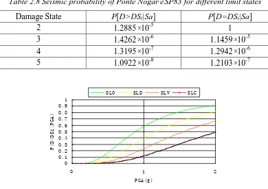
Given (ag)i, from Equation (2.4), the fragility curves of Ponte Nogarè SP83 under

different damage states are calculated as shown in Fig. 2.4. Assuming a spectral

acceleration Sa =0.071g, which is the earthquake intensity with a return period of

475 years, the seismic probabilities of the SP83 Nogarè Bridge in every damage state are calculated as shown in Table 2.8. In table 2.8, the second column gives the probability of exceeding each limit state, and the third column gives the probabilities of exceeding or being in each limit state.

Table 2.7 The required parameters for calculating median spectral accelerations

Damage State t  m (ag)S (g) (ag)L (g) ag (g)

2 0.85 0.6325 0.05 0.5008 0.8829 0.8829

3 0.75 0.6325 0.1 0.4419 1.1728 1.1728

4 0.75 0.6325 0.175 0.4419 1.5515 1.5515

(38)

Table 2.8 Seismic probability of Ponte Nogarè SP83 for different limit states

Damage State P[D>DSi|Sa] P[D=DSi|Sa]

2 1.2885×10-5 1

3 1.4262×10-6 1.1459×10-5

4 1.3195×10-7 1.2942×10-6

5 1.0922×10-8 1.2103×10-7

0 0.1 0.2 0.3 0.4 0.5 0.6 0.7 0.8 0.9 1

0 1 2

PGA(g)

P(D>DSi|PGA)

SLO SLD SLV SLC

Fig. 2.4 Fragility curves of Ponte Nogarè SP83

2.3.2. Example of a bridge with strong bearings and weak piers

The SP90 Bridge on the Adige River at Villa Lagarina is a simply supported, pre-stressed concrete girder bridge with four spans. It was built in 1966. The column parameters are D=1.5m, H=10.45m. The elastic spectra parameters are given in Table 2.9.

(39)

Table 2.9 Spectral parameters at the SP90 Adige Bridge location

Long Lat Sa (Return period of 475 years) Fo Tc S

11.038 45.913 0.116 g 2.484 0.286 1.00

The capacity of the bridge is calculated as the smaller of the two resisting mechanisms, pier collapse or sliding of bearings. If the pier capacity is critical, the capacity coefficient is given by:

c Q p

D

C λ k

H

   (2.15)

Conversely, if sliding of bearings is critical, the capacity coefficient is simply:

t c

C  (2.16)

For computation simplicity, the smaller of the two is used here as the capacity value of this bridge. The parameters of the pier are given in Table 2.10.

Since this is a simple supported bridge, the 3D effects coefficient is given by:

3

3 1 1.08

1 D D

k K

n

  



Table 2.10 parameters of the SP90 Bridge on the Adige River

Damage

states  Q  ag F(PGA)

OLS 0.745 1.0 0.005 0.513 6.66×10-3

DLS 0.674 0.8 0.010 0.718 1.21×10-3

LLS 0.649 0.7 0.020 0.986 1.83×10-4

CLS 0.367 0.6 0.050 1.472 1.16×10-5

0.00 0.10 0.20 0.30 0.40 0.50 0.60 0.70 0.80 0.90 1.00

0 0.5 1 1.5 2 2.5

PGA [g]

P(D

>D

Si

|PG

A)

SLO SLD SLV SLC

(40)

Finally, the fragility curves for the four limit states are given in Fig. 2.6. Similarly, Table 2.11 gives the parameters related with the sliding mechanism, while the corresponding fragility curves are depicted in Fig. 2.7. By comparing the parameters of the two mechanisms, it is evident how in this case the pier mechanism is the more critical, and the corresponding fragility curves are used to represent the bridge vulnerability.

Table 2.11 parameters of the pier

Damage states  t (m) Ai(g) F(PGA)

OLS 0.632 0.85 0.050 1.1124 8.38×10-5

DLS 0.632 0.75 0.100 1.4777 1.13×10-5

LLS 0.632 0.75 0.175 1.9548 1.28×10-6

CLS 0.632 0.75 0.300 2.5595 1.29×10-7

0.00 0.10 0.20 0.30 0.40 0.50 0.60 0.70 0.80 0.90 1.00

0 0.5 1 1.5 2 2.5

PGA [g]

P(D

>D

Si

|PG

A)

SLO SLD SLV SLC

(41)

2.4 Results and conclusions

Using the above methods, the fragility curves for all the bridges in the APT stock are generated. Thus, given an earthquake scenario, seismic vulnerability for all damage states can be calculated, for the same three return periods and four limit states.

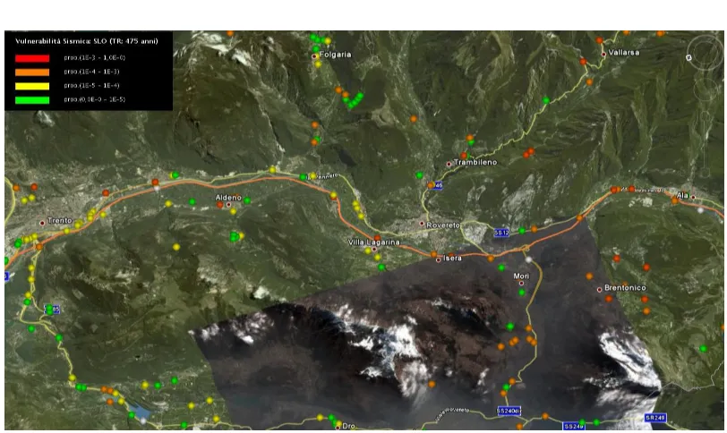
The results with return periods of 475 years, 72 years, and 2475 years are shown in Google Earth maps in Figs 2.8, 2.9, and 2.10 respectively. Bridges are denoted by dots of different colors, according to their probability P of exceeding the limit state: green (P<10-5), yellow (10-5<P<10-4), orange (10-4<P<10-3) and red (P>10-3). This is a very straightforward way to show bridge managers and users the seismic risk of every bridge. The histogram of Fig. 2.11 gives the number of bridges in each probability class for a return period of 475 years.

The results show that the seismic risk for a return period of 475 years in the APT stock is moderate. For limit states OLS and DLS, some bridges have relatively high failure probabilities as shown in Fig. 2.8 (a) and Fig. 2.8 (b). As for limit states LLS and CLS, 99% of the bridges in the APT stock have a very low probability as shown in Fig. 2.8 (c) and Fig. 2.8 (d). This can be explained by the seismic activity of the APT region. Fig 2.12 gives the PGA values of the APT region in the 475 year return period. From Fig. 2.11, we can see that for the 475 year return period, PGA values in most areas of APT region are about 0.075g, which is a very low value. Only in the south east part of APT region, there is a higher PGA value. This region is classified as a low seismic zone.

(a) (b)

(c) (d)

(42)

(a) (b)

(c) (d)

Fig. 2.9 Seismic vulnerability of APT stock for the return period of 72 years in damage states (a), OLS (b), DLS (c), LLS (d), CLS

(a) (c)

(b) (d)

Fig. 2.10 Seismic vulnerability of APT stock for the return period of 2475 years in damage states (a), OLS (b), DLS (c), LLS (d), CLS

(43)

suffering operational problems. It is therefore necessary to identify the safest path between any two given points after an earthquake. Here ‘the safest’ means the lowest risk of exposure to operational problems in a given earthquake scenario. After an earthquake, the ability to decide quickly is of great help to decision makers who need to best distribute the available human and material rescue resources to the disaster center. This problem is addressed in the next section.

0 100 200 300 400 500 600 700 800 900 1000

OLS DLS LLS CLS

Damage state

nu

m

be

r o

f b

rid

ge

s

P<1E-5 1E-5<P<1E-4 1E-4<P<1E-3 P>1E-3

Fig. 2.11 Seismic vulnerability distribution of the APT stock

(44)

2.5 Other methods for generating fragility curves

A review of the literature identified a state-of-the-art method to calculate fragility curves, and I report this here.

2.5.1 The maximum likelihood method (Shinozuka et al. 2000b)

In Shinozuka et al. (2000b), the empirical fragility curves are developed based on the bridge damage data, obtained from the 1995 Hyogo-ken Nanbu (Kobe) earthquake, and on the two-parameter lognormal distribution functions which were used for fragility curve construction. The estimate of the two parameters (median and log-standard deviation) is performed using maximum likelihood method. The peak ground acceleration (PGA) is used to represent the seismic ground motion intensity. The likelihood function is expressed as follows:



 



1

( ) i 1 ( ) i

N

x x

i i

i

L F a F a 





 (2.17)

where F(∙) represents the fragility curve for a specific state of damage; ai = PGA

value to which bridge i is subjected; xi = 1 or 0 depending on whether or not the

bridge sustains the state of damage; and N = total number of bridges inspected after

the earthquake. F(ai) takes the following analytical form:

ln( )

( ) [ ]

a c F a 



(2.18)

where a represents PGA, and [∙] = the standard normal cumulative function. The

two parameters c and in (2) are computed satisfying the following equations to

maximize L:

ln ln

0

d L d L

dc  d  (2.19)

(45)

Impact of Seismic Vulnerability on Bridge Management Systems 0.43) , 0.79 ( MAJOR 0.45) , 0.69 ( MODERATE 0.59) , 0.47 ( MINOR          e e e e e e g c g c g c 0.0 0.4 1.0 0.8 0.6 0.2

0.4 0.5 0.6 0.7 0.8

0.0 0.1 0.2 0.3

PGA(g) P roba bil it y o f E xc ee ding a D amag e S tat e

Fig. 2.13 Example of empirical fragility curves reported by Shinozuka et al. (2000b)

2.5.2 Fragility curves for highway bridges (Karim and Yamazaki 2003)

This method develops analytical fragility curves for highway bridges considering the variation of structural parameters based on numerical simulation. Based on the observed correlation between the fragility curve parameters and the over-strength ratio of the structures, this method constructs the fragility curves using 30 non-isolated highway bridges in Japan, which fall within the same group and have similar characteristics.

It is assumed that there might be a correlation between the fragility curve

parameters and the structural parameters, like the over-strength ratio of the

structure, height of the pier (h), span length (L), and weight (W) of the superstructure.

However, for simplicity, only is considered in the current analysis as it is one of

the key structural parameters and provides information on the reserve strength of the

structure when designed. The over-strength ratio of the structure is defined as:

W k P h e  

 (2.20)

where Pu is the horizontal capacity of the structure, W is the equivalent weight,

which is calculated as the weight of the superstructure and a 50% weight of the

substructure, and khe is the equivalent lateral force coefficient.

1

2 

 a h c h e

k

k (2.21)

(46)

factor of the substructure. The design lateral force coefficient khc is defined as

hco z hc c k

k  (2.22)

where cz is the zonation factor, and khco is the standard design lateral force coefficient.

The value of khco can be obtained by knowing the natural period of the structure and

ground conditions.

The regression model used to obtain the relationship between fragility curves 

and  with the over-strength ratio  is given as:

  

_ b0 b1 (2.23)

  

_ c₀ c₁ (2.24)

where and are the mean and standard deviation of the fragility curves with

respect to ,  is the over-strength ratio of the structure, and b0 and b1 are the

regression coefficients.

2.5.3 Fragility curves for bridge piers based on numerical simulation (Karim and

Yamazaki 2001)

This method presents a numerical analysis to construct fragility curves for bridge piers of a specific bridge based on static sectional and pushover analysis, and non-linear dynamic analysis. The analyses of fragility curves for special piers designed under the 1964 and 1998 Japanese highway bridge codes were constructed with respect to both PGA and PGV. The input motions were selected from the strong records of the 1995 Kobe, 1994 Northridge, 1993 Kushiro and the 1987 Chiba-ken earthquakes.

The steps for constructing analytical fragility curves are as follows.

a. Select the earthquake ground motion records.

b. Normalize PGA of the selected records to different excitation levels.

c. Make an analytical model of the structure.

d. Obtain the stiffness of the structure.

e. Select a hysteretic model for the non-linear dynamic response analysis.

f. Perform the non-linear dynamic analysis using the selected records.

g. Obtain the ductility factors of the structure.

h. Obtain the damage indices of the structure at each excitation level.

(47)

j. Obtain the number of occurrences of each damage rank in each excitation level

and get the damage ratio.

k. Construct the fragility curves using the obtained damage ratio and the ground

motion indices for each damage rank.

For the assessment of the bridge piers, the damage index DI is expressed as

u h d DI

    

(2.25)

where d and u are the displacement and ultimate ductility of the bridge piers,  is

the cyclic loading factor taken as 0.15 and h is the cumulative energy ductility. The

ultimate ductility u is defined as the ratio of maximum displacement (obtained from

the static analysis) to the yield displacement (obtained from the static analysis). The displacement ductility is defined as the ratio of the maximum displacement (obtained from dynamic analysis) to the displacement at the yield point (obtained

from static analysis). The cumulative energy ductility h is defined as the ratio of the

hysteretic energy (obtained from dynamic analysis) to the energy at yield point (obtained from static analysis).

The damage indices obtained for the selected input ground motion are calibrated to get the relationship between the DI and damage rank (DR).

Using the relationship between DI and DR, the number of occurrences of each damage rank is obtained. These numbers are then used to obtain the damage ratio of each damage rank.

To count the number of occurrences of each damage rank, the PGA for selected records were normalized to different excitation levels. Then, the ground motions records were applied to the structure to obtain the damage indices. Using these damage indices, the number of occurrences of each damage rank is obtained for each excitation level. Finally, using the numbers, the damage ratio is obtained for each damage rank.

1.Fragility curves. Fragility curves are constructed with respect to both PGA and

PGV. The damage ratio for each damage rank in each excitation level is obtained by calibrating the DI. Based on this data, fragility curves for the bridge piers are

constructed assuming a lognormal distribution. The cumulative probability PR of the

occurrence of the damage to be equal or higher than rank R, is given as

ln

R

X

P 



  

  _ _ (2.26)

(48)

PGV), and  and  are the mean and standard deviation of lnX. Two parameters of

the distribution are obtained by the least square method on lognormal probability paper. Using these probability papers, the two parameters of the distribution are obtained to construct the fragility curves of the bridge piers.

2.5.4 Seismic fragility methodology for bridges using component level approach

(Nielson and DesRoches 2007)

This methodology considers the contribution of the major components of the bridge, such as the columns, bearings and abutments, to its overall bridge system fragility. In particular, probability tools are used to estimate directly the bridge system fragility from the individual component fragilities.

A probability distribution is developed for the demand, conditioned on the IM, also known as a probabilistic seismic demand model (PSDM), and convolving it

with a distribution for the capacity. The estimate for the median demand (Sd) can be

represented by a power model:

b

d aIM

S  (2.27)

where IM is the seismic intensity measure of choice, and