METHODOLOGY
Quantifying spatial accessibility in public
health practice and research: an application
to on-premise alcohol outlets, United States,
2013
Hua Lu
1*, Xingyou Zhang
2, James B. Holt
1, Dafna Kanny
1and Janet B. Croft
1Abstract
Objective: To assess spatial accessibility measures to on-premise alcohol outlets at census block, census tract, county, and state levels for the United States.
Methods: Using network analysis in a geographic information system, we computed distance-based measures (Euclidean distance, driving distance, and driving time) to on-premise alcohol outlets for the entire U.S. at the census block level. We then calculated spatial access-based measures, specifically a population-weighted spatial accessibility index and population-weighted distances (Euclidean distance, driving distance, and driving time) to alcohol outlets at the census tract, county, and state levels. A multilevel model-based sensitivity analysis was conducted to evaluate the associations between different on-premise alcohol outlet accessibility measures and excessive drinking outcomes. Results: The national average population-weighted driving time to the nearest 7 on-premise alcohol outlets was 5.89 min, and the average weighted driving distance was 2.63 miles. At the state level, population-weighted driving times ranged from 1.67 min (DC) to 15.29 min (Arizona). Population-population-weighted driving distances ranged from 0.67 miles (DC) to 7.91 miles (Arkansas). At the county level, population-weighted driving times and distances exhibited significant geographic variations, and averages for both measures increased by the degree of county rurality. The weighted spatial accessibility indexes were highly correlated to respective population-weighted distance measures. Sensitivity analysis demonstrated that population population-weighted accessibility measures were more sensitive to excessive drinking outcomes than were population weighted distance measures.
Conclusions: These results can be used to assess the relationship between geographic access to on-premise alcohol outlets and health outcomes. This study demonstrates a flexible and robust method that can be applied or modified to quantify spatial accessibility to public resources such as healthy food stores, medical care providers, and parks and greenspaces, as well as, quantify spatial exposure to local adverse environments such as tobacco stores and fast food restaurants.
Keywords: Network analysis, Spatial accessibility, Alcohol outlet
© The Author(s) 2018. This article is distributed under the terms of the Creative Commons Attribution 4.0 International License (http://creat iveco mmons .org/licen ses/by/4.0/), which permits unrestricted use, distribution, and reproduction in any medium, provided you give appropriate credit to the original author(s) and the source, provide a link to the Creative Commons license, and indicate if changes were made. The Creative Commons Public Domain Dedication waiver (http://creat iveco mmons .org/ publi cdoma in/zero/1.0/) applies to the data made available in this article, unless otherwise stated.
Open Access
*Correspondence: [email protected]
1 Division of Population Health, National Center for Chronic Disease Prevention and Health Promotion, Centers for Disease Control and Prevention (CDC), 4770 Buford Highway, N.E. Mailstop F-78, Atlanta, GA 30341, USA
Background
Quantifying spatial accessibility in public health prac-tice is essential for evaluating population exposure to local environments (e.g., alcohol and tobacco outlets or public parks) and population access to health care resources (e.g., primary care clinics or trauma hospi-tals). Three approaches have been reviewed by Zhang et al. [1] and summarized for application to the meas-urement of alcohol outlet density by CDC [2]. Table 1 summarizes the common metrics for quantifying spa-tial accessibility and basic relationships among them. Two commonly used approaches for quantifying spatial accessibility are distance-based and container-based. The spatial interaction (or gravity) model-based spa-tial accessibility index uses both distance-based met-rics and the container concept. Population-weighted accessibility metrics are based on the spatial interaction model-based spatial accessibility index, but at the same time account for the uneven population distribution within a study area. Population-weighted distance met-rics use distance-based metmet-rics and at the same time use the spatial interaction model-based spatial accessi-bility index to construct differential probaaccessi-bility access to destinations and further account for the uneven population distribution within a study area. The most complex population-weighted distance metrics aim to borrow the strengths and at the same time minimize the limits of classic distance-based and container-based metrics, and integrate the power and flexibility of the spatial interaction model-based approach and account for uneven population distributions.
Distance-based measures, such as distance to near-est outlets, are intuitive and relatively easy to generate, but often lack the ability to quantify and incorporate the potential geographic clustering effects of spatial
destinations. The three most common distance-based metrics are listed in Table 1.
The container-based approach is most commonly used to assess outlet density for a predefined area (container). Some common container-based metrics are the number of outlets per square mile or per road mile, or within a predefined spanning distance (Table 1), but often there is an underlying assumption of equal accessibility within this predefined area. There could also be substantial boundary or edge effects, such that outlets near the predefined area boundaries could be either included or excluded in the density calculation. The spatial interac-tion model–based approach assumes the spatial associa-tion or interacassocia-tion between spatial or geographic entities are proportional to their mass sizes and inversely propor-tional to their distances. It takes four basics steps to con-struct a spatial accessibility index, as detailed in Table 1.
The spatial interaction model-based spatial accessibil-ity index is often used by geographers because of its flex-ibility and robustness in quantifying spatial accessflex-ibility. However, interpretations of these indices are not intuitive for public health practitioners and communities. Popula-tion-weighted accessibility (PWA) metrics have similar interpretation challenges in public health practice.
The population-weighted distance (PWD) metrics, a form of spatial accessibility measure developed by Zhang et al. [1] accounts for spatial clustering of outlets, overcomes the unrealistic equal access assumption and potential edge effects of the container-based approach, and also uses an intuitive form of a distance-based meas-ure. In addition, PWD also accounts for uneven popula-tion distribupopula-tion for the geographic area of interest. The flexibility of PWD measures makes them applicable to individual persons or households, as well as for a geo-graphic area. The individual-based PWD measures could
Table 1 Metrics for quantifying spatial accessibility
Distance-based metrics:
Distance to nearest one destination or a group of nearby destinations - Euclidian distance (also known as flight or straight-line)
- driving distance (also known as street network distance, which accounts for street network lengths and connectivity)
- driving time (which further accounts for speed limits for each segment of the street network)
Container-based metrics:
Number of destinations within a pre-specified area or spanning distance or some spatial density measures including but not limited to:
- per 1000 population - per area unit (e.g. square miles) - per road miles
Spatial interaction (gravity) model-based metrics: - Choose distance metrics
- Define distance decay function and distance decay parameter - Specify the destination choice set within an area or spanning distance - Construct spatial accessibility index
Population-weighted accessibility metrics:
Aggregate spatial accessibility index weighted by population - Euclidian distance
- driving distance - driving time
Population-weighted distance metrics:
Use spatial accessibility index to define differential probability access to destinations in the choice set and further weighted by population - Euclidian distance
be applied in specific public health analyses with indi-vidual records. The area-level PWD measures are based on the smallest census geographic units (census blocks); thus, PWD measures could be conveniently aggregated to any larger geographic levels as needed while avoiding the modifiable unit area problem [3]. Despite these poten-tial advantages, PWD measures may be sensitive to the choice of the original distance measures upon which the resulting population-weighted measures are computed. The spatial interaction model to calculate population-weighted accessibility and accessibility index is described in Zhang et al. [1].
In the United States, the census block is the basic unit of census geographic hierarchy (https ://www.censu s.gov/ geo/refer ence/hiera rchy.html). We used census block-level population as our demand area population. By using the population at finest level of census geography that is available in the United States, we minimized the geo-graphic aggregation error for population data described as Source A type of error in Hillsman and Rhoda [4]. Spa-tial access metrics based on higher levels of census geog-raphy than census blocks (e.g. census tract, ZIP Code, or county), even by using population weighted centroids to estimate demand population locations, could still intro-duce substantial spatial aggregation errors or Source A type errors. In addition, the census block-based spatial access metrics provide the flexibility to aggregate the metrics to any high-level geography that could be linked to geocoded individual or aggregated health outcomes. For example, we could easily aggregate census block-based spatial access metrics to higher-level census geo-graphic units, such as census tract, county, ZIP Code, school district, congressional district, or other adminis-trative or customized geographic units, such as hospital service areas, hospital referral regions, and primary care service area. However, there were no studies that quan-tify spatial accessibility based on different census block-level distance measures (Euclidian distance, driving distance and driving time) and evaluate their correlations between population-weighted spatial accessibility index and population-weighted distance metrics.
In this study, we selected on-premise alcohol outlets because of significant public health interest in exces-sive alcohol use. Greater alcohol outlet density is asso-ciated with increased alcohol consumption and related harms [5]. Excessive alcohol consumption is responsible for 88,000 deaths annually in the United States [6] and accounted for $249 billion in economic costs in 2010 [7].
An alcohol outlet is defined as a place where alcohol may be legally sold to a buyer to consume there (e.g., on-premise outlets, such as bars or restaurants) or elsewhere (e.g., off-premise outlets, such as liquor stores) [5]. The on-premise alcohol outlet data that we obtained from
HSIP GOLD is a point dataset that has been geocoded to the street address of the outlets. The point-level data eliminated a location error when geocoding data to ZIP Code area centroid. Regulating alcohol outlet density, which is typically defined as the number of alcohol out-lets in a given area, is an effective strategy for the preven-tion of excessive alcohol consumppreven-tion and related harms [8]. The three general approaches for quantifying spatial accessibility described previously can be applied to the measurement of alcohol outlets [2]. In the container-based approach, the number of alcohol outlets in a given area is calculated. Different denominators can be used as follows: by population size (number of outlets per 1000 population); by area size (number of outlets per square mile); or by road mile length (number of outlets per road mile). Commonly, measurements of alcohol outlet den-sity have used container-based approaches, in which the number of outlets is divided by the population size of a particular area or by the land area itself [9]. However, these approaches could suffer from boundary and edge effects, especially for small geographic areas, and do not directly consider the spatial accessibility between alco-hol outlets and the population [2]. It can result in over-estimates for small areas with large numbers of alcohol outlets, or underestimates for small areas with small numbers or no alcohol outlets.
The distance-based approach calculates the distance to the nearest specified number of alcohol outlets. The distance can be calculated based on Euclidean distance, driving distance through a street network, and driv-ing time through a street network with speed limits. The advantage to this method is that it is intuitive for point-to-point units; however, it is less commonly used in alcohol outlet density studies. The limitation for the distance-based approach is that it ignores the possibility of multiple potential alcohol outlet destinations within an area. An alternative approach is to average the distances to a set of nearest (e.g. five or seven) alcohol outlets. However, this approach suffers from ignoring the une-qual probability of access to any outlet. The population-weighted distance approach uses population as a weight to account for uneven population distributions. It incor-porates unequal probability of access to nearby alcohol outlets, defines the choice set of alcohol outlets guided by human behavioral theory, and is able to account for alco-hol outlet size (if data are available) and spatial clustering [9].
for the entire U.S. Specifically, we use three different dis-tance metrics: Euclidian (flight) disdis-tance, driving disdis-tance and driving time, to construct a spatial accessibility index to generate three population-weighted accessibility met-rics and three more intuitive population-weighted dis-tance metrics. We then compared and evaluated their similarities and correlations. This spatial accessibility modeling framework could be conveniently applied to any other countries or places with hierarchical census geography, such as, census output areas, super output areas, electoral wards, and electoral divisions in the UK; villages, street districts, towns, counties, cities, and prov-inces in China.
Methods Data sources
1. On-premise alcohol outlets
We obtained geocoded data for on-premise alco-hol outlets from the Homeland Security Infrastructure Program (HSIP) GOLD 2013 dataset [10]. It included 210,482 drinking establishments (HSIP terminology to represent on-premise alcohol outlets) in the 50 States and DC, with state averages ranging from 435 (DE) to 16,942 (TX) drinking establishments. The North American Industry Classification System (NAICS) is the standard used by Federal statistical agencies in classifying business establishments for the purpose of collecting, analyzing, and publishing statistical data related to the U.S. business economy. We used NAICS code 7224 and all subcategory NAICS codes of 7224 for Drinking Places (Alcoholic Bev-erages). The types of on-premise alcohol outlets in these NAICS codes include bars and lounges, drinking places, nightclubs, eating places, restaurants, hotels and motels, bowling centers, and recreation clubs. This dataset pro-vided the exact street addresses of on-premise alcohol outlets.
2. Geographic unit of analysis and population demo-graphics
We used 2010 census blocks as our geographic unit of analysis. Census blocks are the smallest unit in the census geographic hierarchy, thus census block-level measures could be aggregated to any geographic levels of inter-est in a very flexible way and minimize the effects of the modifiable area unit problem. We included 6,207,027 census blocks with 2010 populations greater than zero in this study. The geometric centroid of the census block was used to calculate the distance to the location of on-premise alcohol outlets. The 2010 census population count was used as the weight to calculate the population-weighted spatial accessibility index, population-population-weighted driving distance, population-weighted driving time and
population-weighted Euclidean distance at each geo-graphic level.
3. Street network data
We used Esri Data and Maps 10.2 U.S. and Canada Detailed Streets network dataset (Esri, Redlands, CA). These data provide distance and travel times for each street segment that was used in our network analyses.
Measures
1. Distance metrics
We used ArcGIS 10.2.1 Network Analyst (Esri, Red-lands, CA) to calculate the nearest 7 on-premise alcohol outlets for each populated census block. This tool pro-duced a driving distance and a driving time for each ori-gin (census block) and destination (on-premise alcohol outlet) pair. There were 2118 census blocks that did not have access to a street network, and thus were excluded in the driving distance and time calculations. We also calculated the Euclidian distance for each census block to its 7 nearest on-premise alcohol outlets using all cen-sus blocks in the U.S. We used SAS GEODIST func-tion to calculate the Euclidian distance between census block centroids and alcohol outlets (SAS, Cary, North Carolina).
2. Population-weighted spatial accessibility index
We used the spatial interaction model to calculate the population-weighted spatial accessibility index as described in the introduction. Because the size of each on-premise alcohol outlet is unknown, we used a weight of 1 to treat each outlet equally. The Census block-level spatial accessibility index was calculated as:
where i is ith census block, j is jth on-premise alcohol outlet and n = 7 was used for 7 nearest outlets in our
study. The population-weighted spatial accessibility index for geographic units larger than census blocks was calcu-lated as:
where N is the number of census blocks within a geo-graphic area k (e.g. county), Popi is the ith census block’s
Ai= 7
j=1
1
dij
PWAk=
N
total population, and Popk is the total population for the
geographic area k.
3. Population-weighted driving distance/time, Euclidian distance
We used distances and times from the distance-based measures along with block-level populations to calcu-late the population-weighted driving distance and pop-ulation-weighted driving time for each census block. Because of the massive size of the data involved in the study, we stratified the U.S. census blocks into 17 smaller regions for computational purposes to perform the net-work analysis and then merged the results into one data file.
Population-weighted driving distance/time for census block i to 7 nearest on-premise alcohol outlets is calcu-lated as:
where Pij is the probability that a resident at a census block i will choose to visit an alcohol outlet j:
The probability was derived from Huff Model 1963 [11].
Population-weighted driving distance/time for area k is calculated as:
Using these methods, we calculated the weighted accessibility (PWA) index and population-weighted distance (PWD) distances (by driving distance, driving time, and Euclidian distance) to the 7 nearest on-premise alcohol outlets at the census block level. Then, we calculated the same spatial accessibility measures at U.S.-, state-, county- and census tract-levels respectively.
Data analysis
We compared the 6 spatial accessibility measures using Pearson correlation coefficients at the census block level. Specific measures that we analyzed—all at the county level—were driving distance, driving time, and Euclidean distance to the one nearest on-premise alcohol outlet;
PWDi=
j=1∼7
Popi∗Pij∗dij
Popi=
j=1∼7
Pij∗dij
Pij=
1
dij1
7
j=1 1
d1ij =Aij/Ai
PWDk =
N
i=1Popi∗PWDi
PopK
driving distance, driving time, and Euclidean distance to the nearest 7 on-premise alcohol outlets in Aij= 1/(dij^β) with a distance decay parameter β = 1.
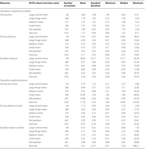
We used county-level spatial accessibility results linked with the 2013 National Center for Health Statis-tics (NCHS) urban–rural classification scheme for coun-ties [12] and calculated spatial accessibility by urban and rural counties to determine whether urban/rural status was associated with spatial accessibility measures. The NCHS urban–rural classification for counties classified U.S. counties into the following 6 categories: (1) large central metro, defined as counties in a metropolitan statistical area (MSA) of at least 1 million residents that contain the entire population of the largest principal city of the MSA, or are completely contained within the larg-est principal city of the MSA, or contain at least 250,000 residents of any principal city in the MSA; (2) large fringe metro, defined as counties in an MSA of 1 million or more residents that does not qualify as a large central metro; (3) medium metro, defined as counties in an MSA of 250,000–999,999 residents; (4) small metro, defined as counties in an MSA of less than 250,000 residents; (5) micropolitan, defined as counties in a micropolitan sta-tistical area; and (6) noncore (often called rural), defined as counties not in MSAs or micropolitan statistical areas. Categories 1–4 are metropolitan counties and categories 5–6 are nonmetropolitan counties.
Sensitivity analysis
their sensitivity to drinking outcomes. A OR larger than one means an increased risk for drinking behaviors, and a larger OR means more sensitive to drinking outcomes. SAS Proc GLIMMIX was used to implement these multi-level logistic models.
Results
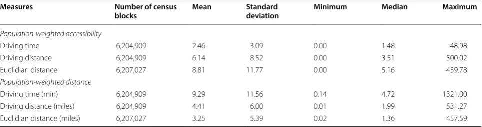
In 2013, the average driving time to the nearest on-premise alcohol outlets (of the nearest 7 choices) for the overall U.S. population was 5.89 min and the average driving distance was 2.63 miles. For all census blocks, the median population-weighted driving time was 4.72 min; population-weighted driving distance was 1.99 miles; and population-weighted Euclidian distance was 1.36 miles (Table 2).
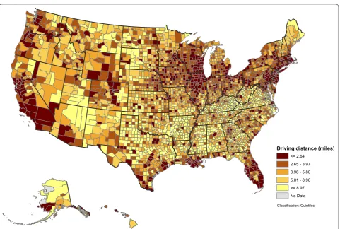
At the state-level (Table 3), population-weighted driv-ing time ranged from 1.67 (DC) to 15.29 min (AR), with a median of 6.67 min (LA); population-weighted driv-ing distance ranged from 0.69 (DC) to 7.91 (AR) miles, with a median of 2.95 miles (LA). In general, states in the northeast, the upper Midwest, and the western U.S. had a driving distance of less than 2 miles to the nearest 7 on-premise alcohol outlets (Fig. 1). The same pattern was observed for driving time (not shown). At the county level, population-weighted driving distance (Fig. 2) and population-weighted driving time (not shown) varied greatly by geography. Shorter population-weighted dis-tances were observed in counties along the northeast coast, around the Great Lakes, in Florida, portions of the Rocky Mountain states, along the west coast, and in large metropolitan areas. Figure 3 presents detailed popula-tion-weighted driving distances at the census tract level. All data for 6 measures at state-, county- and census tract-level are included in Additional file 1.
The mean estimates of population-weighted driv-ing time, drivdriv-ing distance, and Euclidian distance all increased from large central metro to noncore categories (Table 4). Populations living in medium metro counties
had shorter median driving time/distance and Euclidian distance than those living in large fringe metro counties. For the minimum of county-level population-weighted driving time, driving distance, and Euclidian distance, populations living in small metro counties had shorter driving time/distance and Euclidian distance than those living in medium metro counties. Noncore counties had shorter minimum distances than micropolitan counties, for both driving distance and Euclidian distance, but noncore counties had longer minimum driving time than micropolitan counties. For the maximum of county-level population-weighted driving time, driving distance and Euclidian distance, driving time increased with increased rurality; for driving distance, small metro and micropo-litan counties had shorter distances than medium metro counties; small metro counties had shorter Euclidian dis-tances than medium metro counties.
Population-weighted distance measures based on driv-ing time, drivdriv-ing distance, or Euclidian distance were strongly correlated with each other (p < 0.01) (Table 5). Additionally, population-weighted accessibility measures were also strongly correlated with each other (p < 0.01). However, population-weighted distance measures and accessibility measures were moderately correlated to each other (p < 0.01).
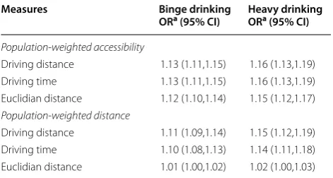
Table 6 presents the odds ratios (ORs) of excessive drinking for an interquartile range increase in popula-tion-weighted accessibility measures and population-weighted distance measures for on-premise alcohol outlets. The interquartile ORs are significantly larger than one, which means that an increased alcohol outlet access were associated with significantly increased risks for excessive drinking in the United States. In other words, the odds ratios represent the minimum risk increase when a person moves from one county with a lower access (first quartile) to alcohol outlets to another county with a higher access (fourth quartile) to alcohol outlets. Population weighted accessibility measures detected
Table 2 Census block-level population-weighted spatial accessibility measures to 7 nearest on-premise alcohol outlets, United States, 2013
Measures Number of census
blocks Mean Standard deviation Minimum Median Maximum
Population-weighted accessibility
Driving time 6,204,909 2.46 3.09 0.00 1.48 48.98
Driving distance 6,204,909 6.14 8.52 0.00 3.51 500.02
Euclidian distance 6,207,027 8.81 11.77 0.00 5.16 439.78
Population-weighted distance
Driving time (min) 6,204,909 9.29 11.56 0.14 4.72 1321.00
Driving distance (miles) 6,204,909 4.41 6.00 0.01 1.99 531.27
Table 3 State-level population-weighted spatial accessibility measures to 7 nearest on-premise alcohol outlets, United States, 2013
State name Census
population 2010
Population-weighted accessibility Population-weighted distance
Driving time Driving distance Euclidian
distance Driving time (min) Driving distance (miles)
Euclidian distance (miles)
Alabama 4,779,736 1.34 3.25 4.93 11.92 5.77 4.02
Alaska 710,231 1.99 5.18 7.54 12.45 5.07 14.19
Arizona 6,392,017 2.46 6.22 9.68 7.33 3.44 2.45
Arkansas 2,915,918 1.20 2.82 4.16 15.29 7.91 5.78
California 37,253,956 3.37 8.51 13.17 3.79 1.56 1.01
Colorado 5,029,196 3.14 7.92 12.18 4.94 2.04 1.37
Connecticut 3,574,097 2.95 6.98 10.59 4.20 1.84 1.22
Delaware 897,934 2.56 6.07 8.93 5.19 2.40 1.66
District of Columbia 601,723 6.92 17.70 25.06 1.67 0.69 0.49
Florida 18,801,310 2.87 7.00 10.75 4.73 1.97 1.26
Georgia 9,687,653 1.66 4.00 6.44 8.71 3.92 2.65
Hawaii 1,360,301 3.19 8.05 11.96 6.73 2.98 2.16
Idaho 1,567,582 2.22 5.72 8.23 7.02 3.02 2.12
Illinois 12,830,632 4.26 10.89 16.61 3.49 1.48 1.02
Indiana 6,483,802 2.44 6.03 8.80 5.96 2.61 1.84
Iowa 3,046,355 3.08 8.07 11.34 5.32 2.25 1.62
Kansas 2,853,118 2.52 6.23 8.88 6.30 2.93 2.14
Kentucky 4,339,367 1.70 4.10 6.39 13.12 6.79 4.55
Louisiana 4,533,372 2.72 6.91 10.72 6.67 2.95 2.01
Maine 1,328,361 1.68 3.92 5.80 10.86 5.25 3.73
Maryland 5,773,552 2.92 7.33 10.78 4.79 2.02 1.31
Massachusetts 6,547,629 3.57 8.73 13.79 3.64 1.57 1.05
Michigan 9,883,640 2.66 6.59 9.41 5.38 2.25 1.59
Minnesota 5,303,925 2.58 6.32 8.92 6.09 2.60 1.85
Mississippi 2,967,297 1.20 2.96 4.37 14.71 7.36 5.44
Missouri 5,988,927 2.50 6.36 9.25 7.10 3.07 2.11
Montana 989,415 2.67 6.80 9.47 8.81 3.99 2.93
Nebraska 1,826,341 3.14 8.10 11.50 5.15 2.22 1.63
Nevada 2,700,551 3.03 7.76 12.96 4.08 1.66 1.11
New Hampshire 1,316,470 1.79 4.21 6.36 8.57 3.88 2.66
New Jersey 8,791,894 4.54 11.49 16.31 3.09 1.32 0.88
New Mexico 2,059,179 1.79 4.30 6.48 10.04 4.91 3.66
New York 19,378,102 5.68 14.94 25.19 2.94 1.21 0.80
North Carolina 9,535,483 1.56 3.83 5.94 9.16 4.11 2.77
North Dakota 672,591 2.67 6.86 9.81 7.92 3.47 2.58
Ohio 11,536,504 3.04 7.55 10.91 5.11 2.23 1.56
Oklahoma 3,751,351 1.89 4.80 6.99 8.61 4.09 2.88
Oregon 3,831,074 3.48 8.75 12.83 4.77 2.05 1.39
Pennsylvania 12,702,379 4.06 10.56 14.86 4.52 1.95 1.32
Rhode Island 1,052,567 4.52 10.82 16.08 2.89 1.29 0.86
South Carolina 4,625,364 1.68 4.11 6.36 7.94 3.48 2.36
South Dakota 814,180 2.44 6.42 8.83 9.11 4.07 3.19
Tennessee 6,346,105 1.56 3.84 5.86 9.78 4.34 2.89
Texas 25,145,561 2.56 6.45 10.00 6.06 2.76 1.91
Utah 2,763,885 1.94 4.66 6.95 6.60 3.03 2.26
stronger associations (larger OR) with excessive drinking outcomes and were more sensitive to alcohol outcomes than population weighted distance measures. Among these spatial accessibility measures, driving distance/ time and Euclidian distance had similar sensitivities to binge drinking/heavy drinking. Among the population-weighted distance measures, driving distance/time-based ones were much more sensitive to binge drinking/heavy drinking than one based on Euclidian distance.
Discussion
Our study has demonstrated a robust approach to quan-tify spatial accessibility of geographic entities from a population health perspective. The population-weighted bottom-up approach provides great flexibility in generat-ing spatial accessibility measures at any geographic level that could be linked with population health outcomes of interest. This is the first nationwide network-based analysis of spatial accessibility to on-premise alcohol out-lets at the level of the census block and their aggregated
Table 3 (continued)
State name Census
population 2010
Population-weighted accessibility Population-weighted distance
Driving time Driving distance Euclidian
distance Driving time (min) Driving distance (miles)
Euclidian distance (miles)
Virginia 8,001,024 1.94 4.65 7.07 8.29 4.01 2.64
Washington 6,724,540 2.98 7.61 11.02 5.30 2.20 1.45
West Virginia 1,852,994 2.02 5.01 7.47 10.69 4.97 3.05
Wisconsin 5,686,986 4.19 10.61 14.74 4.07 1.65 1.15
Wyoming 563,626 2.57 6.50 9.00 7.81 3.56 2.70
Driving distance (miles) 0.69 - 1.95
1.96 - 2.40 2.41 - 3.44 3.45 - 4.11 4.12 - 7.91
Classification: Quintiles
measures provide a more holistic and accurate picture of population spatial accessibility to on-premise alcohol outlets from the local to the national level.
Census block-based population-weighted distance measures are very flexible and can be aggregated to any geographic level as needed (e.g., ZIP Code, neighbor-hood). The method accounts for uneven local population distributions, reduces the ecological bias in measuring alcohol outlet density, and is flexible in that it can incor-porate more information when detailed data are available (e.g. size of the outlets, sales of the outlets). Population-weighted accessibility measures can be linked with other health outcomes at different geographic levels to study the relationship of alcohol access to related harms. Additional analysis is needed to evaluate its sensitivity to excessive drinking outcomes and related population health outcomes. Additional analysis is also needed to evaluate the difference between commercial datasets of licenses alcohol outlets with local alcohol license data.
In spatial interaction modeling and spatial choice mod-eling, how to characterize destination or spatial choice set is still challenging and has no certain answer. We used 7 on-premise alcohol outlets in our model based on Miller
et al. and Saaty et al. [13, 14]. We give different probabili-ties for those 7 outlets based on the Huff model [4]. In this approach, the population in any given census block has a higher probability of accessing a nearer rather than farther on-premise alcohol outlet, and it also accounts for people who may not always chose the nearest outlet.
This study has several limitations. First, alcohol outlet size was treated as one unit (e.g., all alcohol outlets are equally weighted). Second, commercial datasets may not be updated frequently enough to reflect local businesses opening and closing, which may result in over- or under-estimations of spatial accessibility to on-premise alco-hol outlets in some locations. Third, we were aware that people often purchase alcohol from off-premise alcohol outlets (stores) and consume the alcohol at home. Due to lack of data access, we could not include off-premise alcohol outlet in our analysis. This analysis is not meant to present the entire picture of access for both on- and off-premise alcohol outlets. Further analysis may be conducted to include off-premise alcohol outlets in the model to obtain a more comprehensive measure-ment of the impact of alcohol outlet access, once such data becomes available. Finally, census block population
Classification: Quintiles
No Data
Driving distance (miles) <= 2.64
2.65 - 3.97 3.98 - 5.80 5.81 - 8.96 >= 8.97
counts are only available every 10 years when the decen-nial census is conducted. For the non-decendecen-nial years, census block population could be updated via small area population estimation techniques.
Population-weighted spatial accessibility index and population-weighted distance metrics are moderately correlated, which indicates that the population-weighed spatial accessibility index is conceptually different from population-weighted distance metrics and captures dif-ferent aspects or dimensions of spatial accessibility to target destinations. Epidemiologically, we can expect that the population-weighted accessibility measures and population-weighted distance measures could have dif-ferential sensitivity to population health outcomes. Our sensitivity analysis between access to on-premise alcohol outlets and excessive drinking suggested that less-intui-tive spatial accessibility measures are much more sensi-tive than those more-intuisensi-tive direct distance measures. It suggests that some conclusions in the current literature on alcohol outlet density and adverse health outcomes could underestimate the magnitude of associations
between alcohol outlet density and harmful drinking behaviors. These more-sensitive alcohol outlet density measures could be used in public health impact stud-ies on alcohol outlets, provided data with the necessary spatial granularity are available. Alcohol use is a compli-cated human behavior and access to on-premise alcohol outlets is only one of many potential explanatory fac-tors. It is also challenging to quantify people’s preference and selection of on-premise alcohol outlets. Our study method accounts for the probability that closer outlets get more access than more distant outlets, but also takes into consideration that people may not always go to the closest outlets as indicated by a recent USDA report (EIB-138) [15].
Conclusions
These results can be used to assess the relationship between geographic access to on-premise alcohol out-lets and health outcomes. Additionally, this study dem-onstrated a flexible and robust method that can be applied or modified to quantify spatial accessibility to
Classification: Quintiles
No Data
Driving distance (miles)
<= 0.50 0.51 - 1.00 1.01 - 2.00 2.01 - 5.00 5.01 - 10.00 10.01 - 15.00 15.01 - 20.00 20.01 - 50.00 > 50.00
public resources, such as stores that serve healthy food options, medical care providers, and parks and greens-paces, and spatial exposure to local adverse environ-ments such as tobacco stores and fast food restaurants.
This spatial accessibility modeling framework could be conveniently applied to any countries or places with hierarchical census geography. In modern society, cen-sus geographic hierarchy is the base for socioeconomic
Table 4 On-premise alcohol outlets spatial accessibility measures by National Center for Health Statistics (NCHS) urban– rural classification scheme for counties, United States, 2013
Measures NCHS urban/rural class name Number
of counties Mean Standard deviation Minimum Median Maximum
Population-weighted accessibility
Driving time Large central metro 68 4.69 2.38 1.94 4.03 13.31
Large fringe metro 368 1.79 1.03 0.23 1.58 6.92
Medium metro 373 1.91 1.07 0.15 1.86 5.34
Small metro 358 1.91 1.05 0.02 1.97 5.12
Micropolitan 641 1.84 0.92 0.02 1.76 5.59
Noncore 1333 1.27 0.96 0.00 1.01 8.71
Driving distance Large central metro 68 12.02 6.55 4.81 10.06 36.67
Large fringe metro 368 4.39 2.63 0.41 3.94 18.04
Medium metro 373 4.72 2.82 0.22 4.70 14.20
Small metro 358 4.75 2.75 0.11 4.90 12.66
Micropolitan 641 4.52 2.45 0.04 4.26 15.07
Noncore 1333 3.11 2.53 0.00 2.37 19.85
Euclidian distance Large central metro 68 18.40 10.71 7.55 15.11 69.78
Large fringe metro 368 6.57 3.96 0.56 5.83 25.44
Medium metro 373 6.91 4.09 0.28 7.02 19.98
Small metro 358 6.82 3.94 0.35 6.93 17.88
Micropolitan 641 6.29 3.33 0.26 5.98 20.33
Noncore 1335 4.18 3.34 0.00 3.20 24.43
Population-weighted distance
Driving time (min) Large central metro 68 2.79 1.22 0.71 2.75 5.86
Large fringe metro 368 8.94 5.57 1.55 7.51 32.85
Medium metro 373 9.55 6.68 2.31 7.04 44.26
Small metro 358 10.40 7.49 1.85 7.86 48.03
Micropolitan 641 10.88 6.93 2.82 9.09 63.44
Noncore 1333 17.78 11.92 2.94 14.90 216.83
Driving distance (miles) Large central metro 68 1.13 0.50 0.26 1.10 2.49
Large fringe metro 368 4.02 2.84 0.69 3.22 17.55
Medium metro 373 4.56 4.13 0.91 3.09 32.69
Small metro 358 4.92 4.06 0.76 3.43 25.61
Micropolitan 641 5.23 3.90 1.13 4.10 29.61
Noncore 1333 8.97 6.78 0.99 7.07 92.26
Euclidian distance (miles) Large central metro 68 0.73 0.32 0.13 0.68 1.55
Large fringe metro 368 2.71 1.99 0.46 2.18 12.84
Medium metro 373 3.19 3.23 0.61 2.14 26.85
Small metro 358 3.52 3.18 0.51 2.30 20.49
Micropolitan 641 3.80 3.04 0.80 2.95 26.86
and population statistics. Our bottom-up approach within a census geographic hierarchy could be widely applicable and substantially improve the accuracy and flexibility in quantifying population spatial access to public health resources or exposure to environmental hazards of interest.
Abbreviations
CDC: The Centers for Disease Control and Prevention; PWA: population-weighted accessibility; PWD: population-population-weighted distance; HSIP: The Home-land Security Infrastructure Program; NAICS: The North American Industry Classification System; NCHS: The National Center for Health Statistics; MSA: metropolitan statistical area.
Additional file
Additional file 1: Populatiweighted spatial access to 7 nearest on-premise alcohol outlets by U.S. states, counties and census tracts, 2013.
Authors’ contributions
HL, XZ, JBH conceived the study and HL did all the network analysis and made all maps, XZ calculated PWD, PWA and statistical analysis. HL, XZ, JBH, DK and JBC wrote the draft and final version of the manuscript. All authors read and approved the final manuscript.
Authors’ information
The findings and conclusions in this report are those of the authors and do not necessarily represent the official position of the Centers for Disease Control and Prevention or Economic Research Service, U.S. Department of Agriculture.
Author details
1 Division of Population Health, National Center for Chronic Disease Prevention and Health Promotion, Centers for Disease Control and Prevention (CDC), 4770 Buford Highway, N.E. Mailstop F-78, Atlanta, GA 30341, USA. 2 Economic Research Service, U.S. Department of Agriculture, Washington, DC, USA.
Competing interests
The authors declare that they have no competing interests.
Availability of data and materials
The datasets (HISP and Esri Street Network) analyzed during the current study are not publicly available due to data license restriction. Census 2010 block level population can be download at www.censu s.gov. The datasets gener-ated from this study are included in this published article and its additional file.
Consent for publication Not applicable.
Ethics approval and consent to participate Not applicable.
Funding
All authors are U.S. Government employee, therefore the work was founded by U.S. Government.
Publisher’s Note
Springer Nature remains neutral with regard to jurisdictional claims in pub-lished maps and institutional affiliations.
Received: 29 December 2017 Accepted: 19 June 2018
Table 5 Pearson correlation coefficients for the 6 spatial accessibility measures to 7 nearest on-premise alcohol outlets, United States, 2013
All correlations were significant at p < 0.01
Metric Population-weighted accessibility Population-weighted distance
Driving time Driving
distance Euclidian distance Driving time Driving distance Euclidian distance
Population-weighted accessibility
Driving time 1.00 0.97 0.93 − 0.45 − 0.42 − 0.40
Driving distance 1.00 0.95 − 0.41 − 0.39 − 0.38
Euclidian distance 1.00 − 0.43 − 0.41 − 0.34
Population-weighted distance
Driving time 1.00 0.97 0.93
Driving distance 1.00 0.97
Euclidian distance 1.00
Table 6 The odds ratios (ORs) of excessive drinking for an interquartile range increase in population-weighted access measures to nearest 7 on-premise alcohol outlets, United States, 2013
a The ORs were based on an interquartile range scale (the absolute difference
between first and third quartiles), which means the odds increase for risky drinking behaviors when the county-level on-premise alcohol outlet access increases from first quartile to third quartile
Measures Binge drinking
ORa (95% CI) Heavy drinkingORa (95% CI)
Population-weighted accessibility
Driving distance 1.13 (1.11,1.15) 1.16 (1.13,1.19)
Driving time 1.13 (1.11,1.15) 1.16 (1.13,1.19)
Euclidian distance 1.12 (1.10,1.14) 1.15 (1.12,1.17) Population-weighted distance
Driving distance 1.11 (1.09,1.14) 1.15 (1.12,1.19)
Driving time 1.10 (1.08,1.13) 1.14 (1.11,1.18)
•fast, convenient online submission
•
thorough peer review by experienced researchers in your field
• rapid publication on acceptance
• support for research data, including large and complex data types
•
gold Open Access which fosters wider collaboration and increased citations maximum visibility for your research: over 100M website views per year
•
At BMC, research is always in progress.
Learn more biomedcentral.com/submissions
Ready to submit your research? Choose BMC and benefit from: References
1. Zhang X, Lu H, Holt JB. Modeling spatial accessibility to parks: a national study. Int J Health Geogr. 2011;10:31.
2. Centers for Disease Control and Prevention. Guide for measuring alcohol outlet density. Atlanta: Centers for Disease Control and Prevention, US Department of Health and Human Services; 2017. https ://www.cdc.gov/ alcoh ol/resea rch-in-actio n.html. Accessed 30 Aug 2017.
3. Openshaw S. The modifiable areal unit problem. Norwick: Geo Books; 1984.
4. Hillsman EL, Rhoda R. Errors in measuring distances from populations to service centers. Ann Reg Sci. 1978;12:74. https ://doi.org/10.1007/BF012 86124 .
5. Campbell CA, Hahn RA, Elder R, Brewer R, Chattopadhyay S, Fielding J, Naimi TS, Toomey T, Lawrence B, Middleton JC, Task Force on Community Preventive Services. The effectiveness of limiting alcohol outlet density as a means of reducing excessive alcohol consumption and alcohol-related harms. Am J Prev Med. 2009;37(6):556–69.
6. Stahre M, Roeber J, Kanny D, Brewer RD, Zhang X. Contribution of exces-sive alcohol consumption to deaths and years of potential life lost in the United States. Prev Chronic Dis. 2014;11:130293.
7. Sacks JJ, Gonzales KR, Bouchery EE, Tomedi LE, Brewer RD. 2010 National and state costs of excessive alcohol consumption. Am J Prev Med. 2015;49(5):e73–9.
8. Task Force on Community Services. Recommendations for reducing excessive alcohol consumption and alcohol-related harms by limiting alcohol outlet density. Am J Prev Med. 2009;37(6):570–1.
9. Zhang X, Hatcher B, Clarkson L, Holt J, Bagchi S, Kanny D, Brewer RD. Changes in density of on-premises alcohol outlets and impact on violent crime, Atlanta, Georgia, 1997–2007. Prev Chronic Dis. 2015;12:140317. 10. Homeland Security Infrastructure Program (HSIP) https ://www.dhs.gov/
infra struc ture-infor matio n-partn ershi ps. Accessed 20 June 2018. 11. David LH. A probabilistic analysis of shopping center trade areas. Land
Econ. 1963;39(1):81–90.
12. Ingram DD, Franco SJ. 2013 NCHS urban–rural classification scheme for counties. Vital Health Stat 2. 2014;166:1–73. https ://www.cdc.gov/nchs/ data_acces s/urban _rural .htm. Accessed 30 June 2017.
13. Miller GA. The magical number seven, plus or minus: some limits on our capacity for processing information. Psychol Rev. 1956;63(2):81–97. 14. Saaty TL, Ozdemir MS. Why the magic number seven plus or minus two.
Math Comput Model. 2003;38(3–4):233–44.