University of New Orleans University of New Orleans
ScholarWorks@UNO
ScholarWorks@UNO
University of New Orleans Theses and
Dissertations Dissertations and Theses
5-8-2004
Secondary Clarifier Modeling: A Multi-Process Approach
Secondary Clarifier Modeling: A Multi-Process Approach
Alonso Griborio
University of New Orleans
Follow this and additional works at: https://scholarworks.uno.edu/td
Recommended Citation Recommended Citation
Griborio, Alonso, "Secondary Clarifier Modeling: A Multi-Process Approach" (2004). University of New Orleans Theses and Dissertations. 173.
https://scholarworks.uno.edu/td/173
This Dissertation is protected by copyright and/or related rights. It has been brought to you by ScholarWorks@UNO with permission from the rights-holder(s). You are free to use this Dissertation in any way that is permitted by the copyright and related rights legislation that applies to your use. For other uses you need to obtain permission from the rights-holder(s) directly, unless additional rights are indicated by a Creative Commons license in the record and/ or on the work itself.
SECONDARY CLARIFIER MODELING: A MULTI-PROCESS APPROACH
A Dissertation
Submitted to the Graduate Faculty of the University of New Orleans
in partial fulfillment of the requirements for the degree of
Doctor of Philosophy in
The Engineering and Applied Sciences Program
by
Alonso G. Griborio
B.S. University Rafael Urdaneta, 1994 M.S. University of Zulia, 2001
ACKNOWLEDGMENTS
I want to express my deepest gratitude to my adviser, Dr. John Alex McCorquodale, not only for his guidance and support during the development of this dissertation, but also for his patience, his encouragement, and his great ability to transmit ideas. The level of knowledge and expertise that Dr. McCorquodale has showed me during my studies, really impresses me.
I would like to express my special appreciation to Dr. Enrique La Motta, who has been involved in the collection and evaluation of the field data. Thanks for your collaboration.
I would like to thank the rest of my dissertation committee, Dr. Donald Barbe, Dr. Curtis Outlaw and Dr. Dale Easley. The comments and corrections provided by the committee in different chapters of this dissertation are greatly appreciated.
I wish to express my gratitude to Dr. Ioannis Georgiou for his guidance in the elaboration of the TECPLOT files, and his comments in different chapters of the dissertation. Similarly I wish to express my thanks to the people that have been involved in the maintenance of aerobic units at the Marrero Experimental Pilot Plant, Jose Jimenez, Adriana Bustillos, Jackie Luque, and Jose Rojas.
I would like to thank the people that participated at the Clarifier Workshop at Brown and Caldwell’s Walnut Creek office, in special to Dr. Denis Parker and Dr. Eric Wahlberg, for the valuable suggestions in ways to improve the model, and for sharing part of their experience in clarifier design and optimization.
Especially I want to acknowledge to my parents, Alonso and Yudit Griborio, for their incommensurable support, without them, I would not have accomplished this goal.
TABLE OF CONTENTS
LIST OF FIGURES ... xi
LIST OF TABLES... xviii
LIST OF ABBREVIATIONS AND SYMBOLS ... xxii
ABSTRACT... xxix
CHAPTER 1 1 INTRODUCTION ...1
1.1 Background and Problem Definition ...1
1.2 Scope and Objectives...8
1.3 Dissertation Organization ...9
CHAPTER 2 2 LITERATURE REVIEW ...11
2.1 Historical Review of 2-D Modeling of Settling Tanks...11
2.2 Processes in Settling Tanks...20
2.2.1 Flow in Settling Tanks ...20
2.2.1.1 Modeling Equations...23
2.2.2 Settling Properties of the Sludge...27
2.2.3 Turbulence Model...33
2.2.4 Sludge Rheology in Settling Tanks...37
2.2.5 Flocculation Process in Settling Tanks ...41
CHAPTER 3
3 RESEARCH ON SETTLING PROPERTIES. DEVELOPMENT OF A COMPOUND
SETTLING MODEL ...59
3.1 Research on Settling Properties ...59
3.1.1 Study on Wall Effects and Effects of the Stirring Mechanism...60
3.1.2 Study on Discrete Settling ...61
3.1.2.1 Measurement of Discrete Settling Velocities ...63
3.1.2.2 Calculation of the Discrete Settling Fractions ...66
3.1.3 Study on Compression Settling...68
3.2 Development of the Settling Model...70
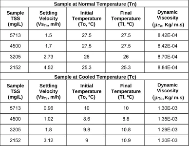
3.3 Effects of Temperature on Settling Velocities...71
CHAPTER 4 4 SETTLING TANK MODEL DEVELOPMENT...76
4.1 Development of Quasi 3D (Q3D) Settling Tank Model...76
4.1.1 Governing Equations ...76
4.1.2 Turbulence Model and Rheology of the Sludge ...81
4.1.3 Settling Model...85
4.1.4 Flocculation Sub-Model...86
4.1.4.1 Shear Induced Flocculation...87
4.1.4.1 Differential Settling Flocculation ...88
4.1.4.2 Transfer of Primary Particles to Flocs in the Flocculation Sub-Model...89
4.1.5.1 Influent Wastewater Temperature and Transport ...91
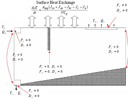
4.1.5.2 Surface Heat Exchange ...92
4.1.6 Scraper Sub-Model ...99
4.2 Numerical Methods...103
4.3 Boundary Conditions ...109
4.3.1 Stream Function Boundary Conditions...109
4.3.2 Vorticity Boundary Conditions...110
4.3.3 Solids Boundary Conditions ...111
4.3.4 Thermal Boundary Conditions...112
4.3.5 Swirl Boundary Conditions...113
4.3.6 Turbulence Model Boundary Conditions...114
CHAPTER 5 5 MODEL CALIBRATION, TESTING AND VALIDATION ...115
5.1 Calibration of the model. Case Study: Marrero WWTP...116
5.1.1 Calibration of the Settling Sub-Model...118
5.1.1.1 Discrete Settling...119
5.1.1.2 Zone and Compression Settling ...123
5.1.2 Calibration of the Flocculation Sub-Model ...127
5.1.3 MLSS, ESS, Flow Rates and RAS...130
5.1.4 Model Simulation...131
5.2 Testing: Grid Dependency Test ...137
5.3 Validation of the Model ...142
5.3.1.1 Marrero WWTP – Early Validation...146
5.3.2 Oxley Creek WWTP ...148
5.3.3 Darvill WWTP New SSTs ...154
CHAPTER 6 6 MODEL APPLICATIONS AND RESULTS...162
6.1 Influence of the Flocculation State on the Secondary Settling Tank Performance ...162
6.2 Flocculation in Secondary Settling Tanks ...164
6.3 Effects of Center Well on Flocculation and Hydrodynamics ...165
6.4 Optimum Dimensions for the Center Well ...169
6.5 Effects of SLR (Constant SOR) on the Optimum Dimensions of the Center Well...174
6.6 Effects of SOR (Constant MLSS, Variable SLR) on the Optimum Dimensions of the Center Well...176
6.7 Solids Flux Limiting Analysis for the Marrero WWTP - Maximum SLR ....178
6.7.1 1D Solids Flux Analysis ...178
6.7.2 Q3D Solids Flux Analysis ...181
6.8 Effect of the SOR on the Performance of the SST – Marrero Case ...185
6.9 Effect of the SOR and the MLSS on the Performance of the SST for a Constant SLR – Marrero Case ...189
6.10 Evaluation of the Different Component of the Flocculation Sub-Model. ...193
6.12 Comparison between Gravity and Rake Induced Flows. Effectiveness of the
Scraper ...199
6.13 Effect of Swirl Components on the Settler Performance...201
6.14 Effect of Temperature and Seasonal Variation on Clarifier Performance...204
6.14.1 Effect of temperature on settling velocity due to change of viscosity ...204
6.14.2 Effect of Influent Temperature Variation and Heat Exchange on the Hydrodynamics and Performance of Clarifiers ...206
6.15 Stability Criteria Analysis...216
CHAPTER 7 7 CONCLUSIONS AND RECOMMENDATIONS ...218
7.1 General Conclusions ...218
7.2 Specific Conclusions...220
7.3 Recommendations...224
REFERENCES ...229
APPENDIX A MARRERO WASTEWATER TREATMENT PLANT...250
APPENDIX B LABORATORY PROCEDURES ...251
APPENDIX C EXPERIMENTAL PILOT PLANT...252
APPENDIX E
RESEARCH ON ZONE SETTLING AND COMPRESSION RATE
PROPERTIES ...264 APPENDIX F
RESEARCH ON TEMPERATURE EFFECTS ON ZONE SETTLING ...280 APPENDIX G
DATA COLLECTED DURING THE VALIDATION OF THE MODEL...288 APPENDIX H
DEVELOPMENT OF THE DIFFERENTIAL SETTLING FLOCCULATION EQUATION...293 APPENDIX I
1DFT ANALYSES ...297 APPENDIX J
FORTRAN SOURCE CODE FOR THE Q3D CLARIFIER MODEL ...307 APPENDIX K
LIST OF FIGURES
Figure 2.1 Flow Processes in a Rectangular Clarifier...21
Figure 2.2 Flow Processes in a Circular Clarifier...23
Figure 2.3 Effective kinematic viscosity of activated sludge ...39
Figure 2.4 Effect of HRT on the SSS removal ...49
Figure 3.1 Solid Liquid Interface Depth vs. Time Using 3 Different Apparatus for a MLSS = 3800 mg/L ...61
Figure 3.2 Sketch of Settling Column...65
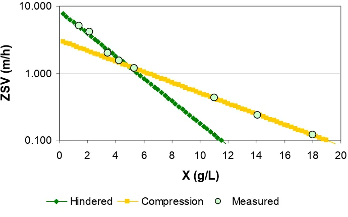
Figure 3.3 Settling Velocities for Hindered and Compression Zone...69
Figure 3.4 Ratios VsT1/ and 2 T Vs 2 T µ /µT1 for Different TSS Concentrations...74
Figure 3.5 Effect of Temperature on Zone Settling Velocity ...75
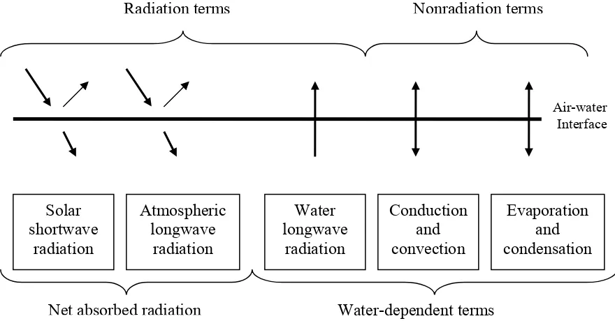
Figure 4.1 The Processes Composing the Surface Heat Exchange ...92
Figure 4.2 Declination Angle, Sine and Cosine of the Declination Angle ...94
Figure 4.3 Local Latitude...94
Figure 4.4 Cosine of the Sun’s Hour Angle...95
Figure 4.5 Albedo of the Water ...96
Figure 4.6 Scheme of Circular Settling Tank for Scraper Definition...100
Figure 4.7 Scheme of Scraper, Tangential and Radial Velocity...101
Figure 4.8 Scheme of Scraper Effect in the θ- direction...103
Figure 4.9 Scalar Control Volume Used for Discretisation Schemes...105
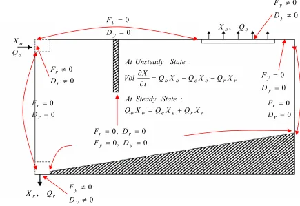
Figure 4.10 Stream Function Boundary Conditions ...109
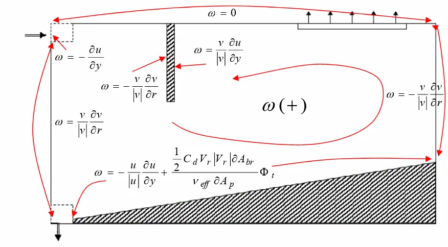
Figure 4.11 Vorticity Boundary Conditions ...110
Figure 4.13 Heat Exchange Boundary Conditions ...112
Figure 4.14 Swirl Boundary Conditions ...113
Figure 4.15 Boundary Conditions for the Simplified Turbulence Model...114
Figure 5.1 Geometry Capabilities of the Model ...116
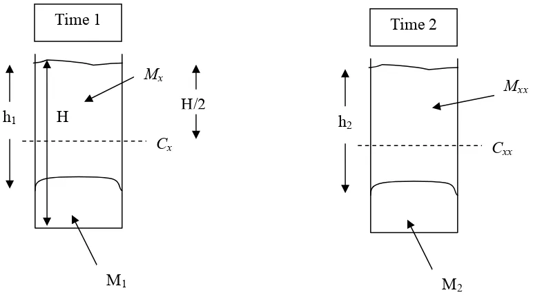
Figure 5.2 Solids-Liquid Interface vs. Time in a Batch Settling Test ...124
Figure 5.3 Field data and Fitted Exponential Equations for Zone Settling and Compression Rate ...126
Figure 5.4 Supernatant SS versus Flocculation Time in a Batch Test...129
Figure 5.5 RAS SS and ESS Concentration Predicted by the Model ...133
Figure 5.6a Concentration Contours at 540 minutes of simulation time for the MarreroWWTP Test Case using a 60x20 grid...134
Figure 5.6b Stream Function and Velocity Vectors at 540 minutes of Simulation Time for the Marrero WWTP Test Case using a 60x20 grid ...135
Figure 5.6c Trajectory Paths and Zones for the 60x20 grid. Marrero WWTP. ...135
Figure 5.7 RAS and ESS Concentrations for Different Grid Sizes ...138
Figure 5.8 Concentration Contours for 3 Different Grids Used in the Marrero Test Case...140
Figure 5.9 Stream Function Contours and Velocity Vectors for 3 Different Grids Used in the Marrero Test Case...141
Figure 5.10 RAS SS and ESS Concentration Predicted by the Model During the Validation...144
Figure 5.12 Measured and Predicted Concentration Profiles at 8.8 m Radial Distance for the Marrero SST ...146 Figure 5.13 Early Validation of the ESS Simulated by the Model...147 Figure 5.14 Flow Rates and Inlet Solids Concentration During at The Oxley Creek
WWTP SST ...150 Figure 5.15 Concentration Contours at 420 minutes of simulation time for the
Oxley WWTP Validation Case using a 40x20 grid ...151 Figure 5.16 Measured and Predicted Concentration Profiles at Different Radial
Distances for the SST of the Oxley Creek WWTP...152 Figure 5.17 ESS, RAS SS and SLR for the Unsteady Simulation of the Oxley Creek
WWTP SST ...153 Figure 5.18 ESS and RAS SS Predicted by the Q3D Model for the Stress Test on the
Darvill WWTP New SSTs ...158 Figure 5.19 Suspended Solids Contours and Velocity Vector for the Four Stress Test
on the Darvill WWTP New SSTs ...159 Figure 6.1 ESS for Three Study Cases with Different Initial Discrete Settling
Fractions...163 Figure 6.2 ESS for 4 Study Cases in Center Well Effects ...166 Figure 6.3 Concentration Contours and Velocity Vectors for the Marrero SST with
Figure 6.5 Effect of Center Well Radius on Clarifier Performance (Baffle Depth = 2.6m, SOR = 1 m/h, SLR= 4.20 kg/m3, RAS = 50%) ...169 Figure 6.6 Effect of Center Well Radius on the Clarifier’s Flow Pattern (Baffle Depth = 2.6m, SOR = 1 m/h, SLR= 4.20 kg/m3, RAS = 50%) ...170 Figure 6.7 Effect of Center Well Depth on the ESS (Baffle Radius = 5.0 m, SOR = 1 m/h, SLR= 4.20 kg/m3, RAS = 50%) ...171 Figure 6.8 Effect of Center Well Depth on the Clarifier’s Flow Pattern (Baffle Radius = 5.0 m, SOR = 1 m/h, SLR= 4.20 kg/m3, RAS = 50%) ...172 Figure 6.9 Comparison of Two Different Center Well Depths under Extreme Loading Conditions (Baffle Radius = 4.5 m, SOR = 2.5 m/h, MLSS = 2. kg/m3, RAS = 50%)...173 Figure 6.10 Flow Pattern and SS Contours for Two Different Center Well Depths
under Extreme Loading Conditions (Baffle Radius = 4.5 m, SOR = 2.5 m/h, MLSS = 2.8 kg/m3, RAS = 50%) ...174 Figure 6.11 Effect of SLR on Optimum Position of the Center Well (Baffle Depth = 2.6m, SOR = 1 m/h, SLR= Variable; RAS = 50%) ...175 Figure 6.12 Effect of SOR on Optimum Position of the Center Well (Baffle Depth = 2.6m, MLSS = 2.8 Kg/m3, SLR= Variable, RAS = 50%) ...176 Figure 6.13 Optimum Center Well Radius versus SOR (Baffle Depth = 2.6m, MLSS = 2.8 Kg/m3, SLR= Variable, RAS = 50%) ...177 Figure 6.14 Flow Pattern and SS Contours for a Large Center Well under Different
Figure 6.15A 1D Solids Flux Analysis for the Marrero WWTP using the Zone Settling Properties ...179 Figure 6.15B 1D Solids Flux Analysis for the Marrero WWTP using the Zone Settling and Compression Rate Properties (Vo= 10.54 m/h, K1= 0.40 L/g, Vc= 3.20
m/h, Kc= 0.184 L/g) ...180
Figure 6.16 ESS vs SLR. Limiting Solids Flux Analysis (SOR= 1 m/h, UFR= 0.5 m/h, MLSS= Variable, RAS =50%) ...182 Figure 6.17 Sludge Blanket Position for Limiting and Failing SLRs (SOR= 1 m/h,
UFR= 0.5 m/h, MLSS= Variable, RAS = 50%) ...184 Figure 6.18 ESS vs SOR. Limiting Solids Flux Analysis (SOR= Variable, UFR=
0.5xSOR, MLSS= 2.8 Kg/m3) ...186 Figure 6.19 Influence of SOR in the Flow Pattern and the Position of the Sludge
Blanket (SOR= Variable, UFR= 0.5xSOR, MLSS= 2.8 Kg/m3)...188 Figure 6.20 Performance of the SST for a Constant SLR and Variables SOR and
MLSS (SOR= Variable, UFR= 0.5xSOR, MLSS= Variable, SLR= 4.20 Kg/m2.h)...190
Figure 6.23B Flat Bed Clarifier with Suction Withdrawal System – Lower RAS Ratio (Depth = 5.0m, SOR= 1.0 m/h, UFR= 0.3 m/h, MLSS= 2800mg/L)...197 Figure 6.24 Oscillation Presented in the RAS SS and ESS Concentration with the
Simulation of the Rake Type Scraper ...198 Figure 6.25 Horizontal Velocities in a Gravity Flow for a Sloping Bed Circular
Clarifier (Bottom Slope= 8.33)...199 Figure 6.26 Horizontal Velocities in a Gravity Flow for a Sloping Bed Circular
Clarifier and Comparison with the Radial Velocities of the Scraper (Bottom Slope= 8.33%, Scraper Velocity= 0.033 rpm, Blade Angle= 45º).. ...201 Figure 6.27 Simulated Velocity Gradients with and without Inlet Deflector (SOR= 1.0 m/h) ...203 Figure 6.28 Predicted ESS and RAS SS Concentrations with Settling Properties Corrected for Different Temperatures due to Change of Viscosity...206 Figure 6.29 Effect of Influent Temperature Variation on the ESS Concentration (SOR= 1.0 m/h, MLSS= 2800 mg/L) ...208 Figure 6.30 Effect of Influent Temperature Variation on the Suspended Solids
Figure 6.33 Effect of Seasonal Variation on the Performance of the SST (SOR= 1.0 m/h, MLSS= 2800 mg/L)...213 Figure 6.34 Effect of Surface Cooling on the Suspended Solids Contours ...214 Figure 6.35 Temperature Stratification under the Effect of a Surface Cooling Process
LIST OF TABLES
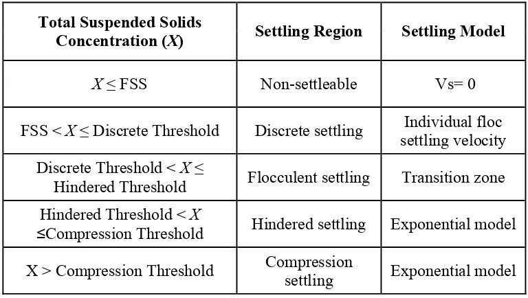
Table 3.1 Settling Regions Based on the TSS Concentration...70
Table 3.2 Settling Velocities and Dynamic Viscosities for Samples at Normal and Cooled Temperature...73
Table 3.3 Ratios VsT1/ and 2 T Vs 2 T µ /µT1 for Different Samples...74
Table 4.1 Settling Velocities and Cross Sectional Diameters for Different Particle ..89
Table 5.1 Dimensions and Operating Characteristics of the SST at the Marrero WWTP ... 117
Table 5.2 MLSS, RAS and Threshold Concentration...118
Table 5.3 Discrete Settling Velocities of Large Flocs ...119
Table 5.4 Discrete Settling Velocities of Medium Flocs...120
Table 5.5 Data for the Calculation of the Discrete Settling Velocity of Small Flocs... ...121
Table 5.6 Data for the Calculation of the Discrete Settling Fractions ...122
Table 5.7 Discrete Settling Velocities and Fractions...123
Table 5.8 Field Data for the Determination of the Settling Parameter of the Zone Settling and Compression Rate Exponential Equations...125
Table 5.9 Calibrated Settling Parameter of the Hindered and Compression Settling Equations...126
Table 5.10 Kinetic Constant for the Flocculation Sub-Model...129
Table 5.11 Suspended Solids Concentrations Measured During the Calibration Period . ...130
Table 5.13 Input Data for the Clarifier Model Simulation ...132
Table 5.14 Comparison between Measured and Predicted Values for Calibrated Model ...133
Table 5.15 Grid Sizes Evaluated in the Dependency Test...137
Table 5.16 ESS and RAS SS Concentrations at Equilibrium Conditions for 3 Grid Sizes ...139
Table 5.17 Suspended Solids Concentrations Measured at the Marrero WWTP During the Validation Period...142
Table 5.18 General Data for the Validation of the Q3D Model – Marrero WWTP ...143
Table 5.19 Comparison between Measured and Predicted Values During the Validation of the Q3D Model ...144
Table 5.20 Settling Properties (Takacs’ Model) for the Oxley Creek WWTP...148
Table 5.21 Summary of Oxley Creek WWTP SST Characteristics ...149
Table 5.22 Predicted and Measured ESS and RAS SS Concentration Under Steady State Conditions for the Oxley Creek WWTP SST Simulation ...151
Table 5.23 Geometry of Darvill WWTP New SSTs...155
Table 5.24 Summary of the Four SLR Stress Test Done on the Darvill WWTP New SSTs ...155
Table 5.25 1 DFT Predicted Maximum SOR ...156
Table 5.26 Darvill WWTP New SST Stress Test Results ...156
LIST OF ABBREVIATIONS AND SYMBOLS
Abbreviations
1D, 2D, 3D One-, two- and three dimensional ADI Alternating direction implicit AS Activated sludge
CCOD Colloidal COD
CFD Computational fluid dynamics CFSTR Continuous flow stirred tank reactor COD Chemical oxygen demand
CRTC Clarifier research technical committee DCOD Dissolved COD
DO Dissolved oxygen DSS Dispersed suspended solids EESS Excess effluent suspended solids EPS Extracellular polymeric substance ESS Effluent suspended solids
FCW Flocculation center well FDM Finite difference method FEM Finite element method FSS Flocculated suspended solids FTC Flow-through curves FVM Finite volume method FW Flocculation well
HLPA Hybrid linear-parabolic and oscillation-free convection scheme HRT Hydraulic retention time
ISS Influent suspended solids KE Kinetic energy
PDE Partial differentials equation PE Potential energy
PST Primary settling tank
Q3D Quasi 3-dimensional clarifier model
QUICK Quadratic upstream interpolation for convective kinematics RAS Return activated sludge, recycle ratio
SIM Strip integral method SLR Solids loading rate SOR Surface overflow rate SRT Sludge retention time SS Suspended solids
SSS Supernatant suspended solids SST Secondary settling tank
ST Settling tank
SVD Settling velocity distribution TCOD Total COD
TDS Total dissolved solids
TF/SC Trickling filter-solids contact processes TSS Total suspended solids
UFR underflow rate
WWTP Wastewater treatment plant ZSV Zone settling velocity
Symbols English
A area
Albedo, Equation 4.29
As clarifier superficial area
Β settling parameter for Equation 2.17 opening height, Equation 2.51 b fitting parameter, Equation 2.16
C concentration of unflocculated particles
D
C drag coefficient
p
C specific heat
O
C initial concentration of influent particles c fitting parameter, Equation 2.16
d fitting parameter, Equation 2.16 D fractal dimension
diameter of the inlet, Equation 2.50 da size of the aggregate
dp diameter of the particle Ε porosity
Ea atmospheric emissivity
e
air vapour pressureF force
f discrete settling fraction
partition function, Equation 3.1 G means square velocity gradient
g vertical component of the gravitational acceleration h vertical distance
Hb height of the blade on the scraper submodel Io insolation at outer limit of earth’s atmosphere k settling parameter
Jshe total surface heat flux
Jan atmospheric longwave radiation
Jbr water longwave radiation
Jcc heat transfer due to conduction and convection
Jec heat transfer due to evaporation and condensation
K settling parameter k turbulence kinetic energy
kc settling parameters for the compression settling model
k1 settling parameters for the zone settling
settling parameters of the hindered settling zone for the Takacs model k2 settling parameter for the low solids concentration region
kf flocculation constant, Equation 2.39
KA floc aggregation coefficient
KB floc breakup rate coefficient
Lf longest dimension of the floc
lm mixing length
M mass
m settling constant for Cho model
coefficient for cylindrical or Cartesian coordinates in Equations 2.1 to 2.6 stress growth exponent, Equation 2.34
floc break up rate exponent, Equation 2.35 relative thickness of air mass, Equation 4.27 N number of arm in the scraper submodel
Fraction of the sky obscured by clouds, Equation 4.28
n
primary particle number concentration n settling constant for Cho model (Chapter 2)non-Newtonian exponent (Chapter 2) turbidity factor of the air, Equation 4.27 NR Reynolds number
p hydrostatic pressure
P total energy loss or power imparted to the water
Po empirical coefficient, Equation 2.22 Q air-flow rate
Qe,Qeff effluent flow rate Qi influent flow rate
q fitting parameter, Equation 2.16 r radius
So specific surface area
Ss particle specific gravity
T temperature
Td dew point temperature Tsw water surface temperature Uw wind speed
u velocity along r- and x- coordinate v velocity along y- coordinate
V reactor volume
Vbr velocity of the blade in the radial direction
Vo settling parameter Vc compression rate parameter Vs particle settling velocity
Vsp terminal settling velocity of the primary particle Vt tangential velocity solids
Wbo solar constant
X concentration of suspended solids Xd threshold for discrete settling Xh threshold for hindered settling Xc threshold for compression settling
Xmin minimum attainable settling concentration
z cloud base-altitude, Equation 4.28
Greek
νsr eddy diffusivity of suspended solids in the r-(x) direction
νt eddy viscosity
σ Stefan-Boltzmann constant
σsr Schmidt number in the r-(x) direction σsy Schmidt number in the y-direction
µ fluid dynamic viscosity ν kinematic viscosity
Θ settling parameter, Equation 2.17
Γ settling parameter, Equation 2.17
Γr effective diffusion coefficient in the r- direction
Γy effective diffusion coefficient in the y- direction
ε the rate of energy dissipation emissivity of water, Equation 4.31 λ Kolmogorov microscale
overall primary particle removal rate, Equation 2.38 molecular diffusivity, Equation 2.58
φ solids fraction ρf floc density
φg gel solids fraction ρp particle density ρ, ρl fluid density ρr reference density
τ shear stress τo yield stress
τ sun’s hour angle ηp plastic viscosity
γ* magnitude of the strain rate
angle of the radiation with the horizon
β removed primary particle concentration, Equation 2.38
β (a,p) collision frequency function between the aggregate and small particles
κ permeability of the aggregate
θ
v velocity components in the θ- directions respectively νeff effective viscosity
ω vorticity
ψ stream function
Ω scraper angular velocity
α equilibrium primary particle number concentration recycle ratio
angle of the radiation with the horizon λ Kolmogorov microscale
overall primary particle removal rate, Equation 2.38 molecular diffusivity, Equation 2.58
δ declination angle
ABSTRACT
The performance of settling tanks depends on several interrelated processes and factors that include: hydrodynamics, settling, turbulence, sludge rheology, flocculation, temperature changes and heat exchange, geometry, loading, the nature of the floc, the atmospheric conditions and the total dissolved solids concentration. A Quasi-3D (Q3D) clarifier model has been developed to include the following factors: axisymmetric hydrodynamics (including the swirl component), five types of settling (nonsettleable particles, unflocculated discrete settling, flocculated discrete settling, hindered settling and compression), turbulence, sludge rheology, flocculation with four classes of particles, temperature changes and surface heat exchange with the atmosphere, various external and internal geometry configurations, unsteady solids and hydraulic loading, the nature of the floc settling/interaction. The model includes: shear flocculation, differential settling flocculation and sweep flocculation. The Q3D model reproduces the major features of the hydrodynamic processes and solids distribution on secondary clarifiers. When the model is executed with the field derived settling characteristics, it can accurately predict the effluent and recirculation suspended solids concentrations. The model has been formulated to conserve fluid, tracer and solids mass.
The model has been developed and tested using field data from the UNO Pilot Plant and the Jefferson Parish Waste Water Treatment Plant located at Marrero, Louisiana. A field testing procedure is presented that addressees all of the settling regimes that are encountered in a Secondary Settling Tank.
CHAPTER 1
1 INTRODUCTION
1.1Background and Problem Definition
“The bottle neck limiting the capacity of the wastewater treatment plant” (Ekama and Marais, 2002), “the most sensitive and complicated process in an activated sludge treatment plant” (Ji et al., 1996), “almost invariably the reason for poor performance of an activated sludge system” (Wahlberg et al., 1995); these are just a few examples of expressions emphasizing the role of the secondary clarifier in the overall performance of the activated sludge system. Already critical in conventional biological treatment systems; the new treatment tendencies based on pollutant size distribution [e.g. role of bioflocculation on COD removal, La Motta et al. (2004a)] further stress the importance of secondary settling tanks (SST). In suspended growth systems, such as conventional activated sludge (AS), dissolved, colloidal and even a portion of particulate contaminants have been converted (i.e., oxidize in the biological-aeration tank) into suspended microbial mass, water and biogases. The SST has the responsibility of the physical separation of the microbial mass and remaining settleable particles from the liquid (i.e., clarification function).
and transported to the biological reactor (i.e., thickening function). A fourth, usually overlooked, function should be added: storage. The SST has to allow for accumulation of sludge during peak flows, but also for accumulation of sludge due to system operation (e.g., when the wasted sludge is less than the biomass produced daily, solids accumulation will occur in the biological reactor, in the SST or in both). Although it is commonly assumed that the sludge purged from the system is equal to the produced biomass, La Motta et al. (2004b) found that sludge accumulation is very likely to occur under typical operating conditions.
The performance of SST depends on several interrelated processes; for simplicity, these processes have been divided into six groups: (A) hydrodynamics, (B) settling, (C) turbulence, (E) sludge rheology, (F) flocculation, and (G) heat exchange and temperature changes. At the same time, these processes depend on numerous, also interrelated factors, that include: (1) the geometry of the tank, including inlet and outlet configurations, sludge withdrawal mechanisms, internal baffles and bottom slope; (2) loading, including solids and hydraulic loading, and time variations; (3) the nature of the floc in the mixed liquor suspended solids (MLSS), including the settling properties and the tendency to aggregation and break up; (4) the variations in the total dissolved solids (TDS); (5) the atmospheric conditions, including ambient and water temperature, shortwave and longwave radiations, and wind. Naturally, the weight of these processes and factors is variable, and therefore neglecting assumptions can be made. However, a complete model for SST must include sub-models for the six aforementioned groups, allowing for the representation of the interrelated factors. Obviously this is not an easy task, and so far it has not been completed (to the knowledge of the author).
are included in the tank, which should optimize the clarification efficiency. This second stage is usually done following some semi-empirical rules (e.g., twenty minutes retention time in the flocculator center-well) and strongly relies on the engineer’s experience. Ekama et al. (1997) concluded that the predicted maximum permissible solids loading rate, using the 1DFT, over-predicts the permissible solids loading rate (SLR) by about 25%. However, there was no convincing evidence that an 80% reduction in the predicted SLR needed to be applied for all SST (Ekama and Marais, 2002). Definitely, different tank geometries and configurations might give different correction factors.
1D models do not account for the major features in tank hydrodynamics and internal configurations; this has to be done at least in a 2D layout. Several 2D models of various complexities have been developed for simulating circular and rectangular, primary and secondary settling tanks. A detailed historical review will be presented in Chapter 2 but a state of the art review in 2D modeling will now be presented.
The first 2D clarifier model was presented by Larsen (1977). His model, developed for rectangular clarifiers, was based on the equations of motion, continuity and an exponential equation relating settling velocity to concentration. He introduced the concept of stream function and vorticity, and the generation of vorticity by internal density gradients and shear along solid boundaries. Diffusivity was assumed equal to eddy viscosity, which was computed on the basis of the Prandtl mixing length theory.
McCorquodale, 1985b) coupling the hydrodynamics with a transport model to simulate the transport and settling of primary particles in circular settling tanks; the model was restricted to the neutral density case. Celik et al. (1985) presented a numerical finite-volume method (FVM) using the k-ε turbulence model for predicting the hydrodynamics and mixing characteristics of rectangular settling tanks. Devantier and Larock (1986, 1987) introduced a Galerkin finite element method to model a steady two-dimensional flow in a circular SST. They modelled the sediment-induced density current in the circular clarifier but did not model the inlet region.
McCorquodale et al. (1991) introduced a numerical model for unsteady flow in a circular clarifier. The model included a description of density currents in the settling zone only. The authors introduced the double-exponential settling velocity formula of Takacs et al. (1991), which allows for a lower settling velocity in a low-solids concentration region. Although this equation was developed for one-dimensional settling tank modelling, it has been widely used in 2D modelling since then.
Zhou and McCorquodale (1992a, 1992c,) presented a numerical and computer model for unsteady flow in a center-fed secondary circular clarifier that included simulation of the inlet zone. At that time, they (McCorquodale and Zhou, 1994a) concluded that numerical models were sufficiently well advanced so that they could be used as a tool in the selection of critical tank dimensions such as depth, diameter, launder locations, bottom slope and skirt dimensions.
Lately, Zhou et al. (1994) used a numerical model to investigate the unsteady flow regime and the temperature mixing in temperature-stratified primary rectangular settling tanks. They introduced an equation of state for the local fluid density as a function of temperature, and a convection-diffusion equation to determine the temperature field in the tank.
et al. (1992) developed a 2D steady state model to simulate the settling of discrete particles in rectangular tanks with a settling velocity distribution (SVD). The model, which accounted for the effects of sediment-induced density currents, included a simple approach to describe flocculation. The flocculation model assumed only turbulent shear-induced flocculation. Szalai et al. (1994) included swirl effects into a circular tank. The calculations were restricted to steady state and neutrally buoyant case. Dahl et al. (1994) presented a steady state model that took into account the rheology of the activated sludge; it included the Bingham plastic characteristic of activated sludge suspensions.
Ji et al. (1996) coupled a 2D clarifier model to an aerobic biological reactor. The coupling arrangement was used to simulate the response of the system to the change of the return activated sludge ratio (RAS) under steady-state influent and investigate the possible remedial actions for peak wet weather flow conditions for a dynamic influent. Vitasovic et al. (1997) used data, collected by Wahlberg et al. (1993) through application of the Clarifier Research Technical Committee (CRTC) protocol, to perform simulations of the Denver secondary clarifier. They tested different loadings and settling properties, and introduced modifications in the tank geometry (decreased the size of the flocculation center well and added a Crosby baffle) that improved the hydrodynamics and tank performance.
Lakehal et al. (1999) and Armbruster et al. (2001) presented a model for unsteady simulation of circular clarifiers that included the sludge blanket in the computation domain. A rheology function was included that accounted for the increased viscosity of highly concentrated sludge mixtures. Stamou et al. (2000) applied a 2D mathematical model to the design of double-deck secondary clarifier. They modelled each tank independently adjusting the boundary conditions for the independent cases.
results of the 1D and 2D approaches were compared with full-scale stress tests. Settler-CAD accurately predicted the results of 12 of 15 selected tests.
In recent years, CFD commercial programs have become fast and user-friendly and have been widely used by engineers in many fields. Two of the most common CFD packages are PHOENICS and FLUENT. Examples of PHOENICS applications can be found in Krebs (1991), Dahl et al. (1994), Krebs et al. (1995), De Cock et al. (1999) and Brouckaert and Buckley (1999). Laine et al. (1999), De Clercq (2003), and Jayanti and Narayanan (2004) used FLUENT for their simulation of the 2D hydrodynamics of settling tanks. De Clercq presented an extensive study in SSTs that included calibration and validation with both lab-scale and full-scale investigations. He implemented submodels that account for the rheology of the sludge, the Takacs solids settling velocity and the scraper mechanism.
models. Even though very little information about 3D models has been published, the limitations presented in this paragraph about 2D models extend to 3D models, with the exception of swirl effect simulation.
The discussion presented so far is summarized as follows:
• Secondary clarifiers play a major role in the overall wastewater treatment plant performance. SST should be designed at least with the same level of detail and expertise as is used to design the biological process.
• Although a very complex problem, SSTs are designed with many simplifications. The most common way of designing a SST is the 1DFT model, which seems to over-predict the permissible solids loading and does not account for the major hydrodynamic features of the tanks. Internal geometry, which may control the clarification efficiency of the clarifier, can not be evaluated using 1D models. The internal features are usually added following semi-empirical rules and are based on engineering experience.
It can be concluded from the discussion that the current ways in which SSTs are designed and modified could and should be improved. Providing a tool that might lead to clarifier optimization, as well as understanding, quantifying and visualizing the major processes dominating the tank performance, are the main goals of this research.
1.2Scope and Objectives
This research focuses on the development of a Quasi-3D model (Q3D model) that can be used as an aid in the design, operation and modification of secondary clarifiers. This model represents in a 2D scheme the major physical processes occurring in SSTs. However, swirl effects due to rotating scrapers and inlet vanes are also included, hence the Quasi-3D definition. Obviously, such a model can be a powerful tool; it might lead to clarifier optimization, developing cost-effective solutions for new sedimentation and flocculation projects and helping existent clarifiers to reach new-more demanding standards with less expensive modifications. An important benefit is that the model may increase the understanding of the internal processes in clarifiers and their interactions, e.g., clarifying the role of flocculation on the tank performance. A major goal is to present a model that can be available to the professionals involved in operation, modification and design of clarifiers; in this respect, the model was developed following two premises: first; a non-commercial code for the solver was developed, i.e., no commercial CFD program was used to avoid the high cost of this type of software; second, the recalibration of the model for the application to specific cases was designed to be as straightforward as possible, i.e., whenever possible the theory with the simplest calibration parameters was used. The specific objectives of this research include:
• Develop an appropriate relationship for the simulation of the settling velocities on the entire curve of suspended solids usually encountered in SST.
• Introduce a flocculation submodel in the general SST model, including surface heat exchange.
• Introduce a temperature submodel in the general SST model.
• Develop a model calibration procedure, including the calibration of the settling properties and flocculation submodels.
• Evaluate the grid and time dependency of the model solution.
• Evaluate the role of the different submodels (e.g. settling properties, flocculation, temperature, and rheology) in the SST prediction.
1.3Dissertation Organization
This document is organized into six chapters:
Chapter 1 introduces the topic, presents a short description about clarifier modeling, and discusses the problem, the dissertation scope and objectives, and the organization of the document.
Chapter 3 presents the research on settling properties that led to the development of a compound settling model. A study about the effects of temperature on the settling properties is also presented in this chapter.
Chapter 4 demonstrates the development of the Quasi 3D mathematical model. This chapter introduces the governing equations, the turbulence and rheology submodels, and the scraper submodel that are used in the model. Chapter 3 presents a short review in numerical methods and a discussion about the methods used in this research to discretise and solve the differential equations.
Chapter 5 discusses the calibration of the model, including the calculation of all the parameters needed for the calibration. This chapter also includes a grid dependency test and the validation of the model with three different test cases.
Chapter 6 presents several applications of the model. The results of these applications are discussed in this chapter.
Chapter 7 states the general and specific conclusions of the research. Recommendations for improving the model and future research are also presented in this chapter.
CHAPTER 2
2 LITERATURE REVIEW
2.1 Historical Review of 2-D Modeling of Settling Tanks
The clarifier modeling field has its beginning in 1904 when Hazen introduced the overflow rate concept, a design concept which has been widely used and still is a major criterion in settling tank design. Hazen’s theory states that the hydraulic retention time should be equal to the time needed for a particle to settle from the top to the bottom of the tank; in this way all the particles with settling velocities higher than that of the design particle will be removed. Hazen’s theory has many assumptions that make its application unrealistic for secondary settling tanks: (1) Hazen assumes a uniform horizontal velocity field where turbulence is not considered; in reality, the flow field in SST is turbulent and heterogeneous in nature, and the high solids loading and low hydraulic loading lead to density-dominated flows. The relationship between hydraulic efficiency and removal of suspended solids cannot be clearly understood unless the influences of density differences on the hydrodynamics are considered (Zhou and McCorquodale, 1992a). (2) Hazen assumes that the settling rate of the particle is constant and is independent of the flow; this can be true for discrete particles settling, but in SST the flocculent, hindered and compression settling usually dominate the process, and these are influenced by the concentration of suspended solids and the biological nature of the flocs. Also, flow and sedimentation strongly interact via density effects and flocculation or floc break up (Ekama et al., 1997). In large grit chambers and primary settling tanks Hazen’s assumptions can be approximately valid and useful to represent the process.
Dobbins (1944) and Camp (1945, 1952) introduced analytical solutions that allowed vertical mixing to be included in a Hazen type model. The analysis presented by Dobbins was based on the concept of overflow rate using a plug flow assumption and accounted for the effects of wall-generated turbulence on sedimentation. Camp approximated the effect of turbulence in retarding settling. In general, their theories expanded the knowledge of the sedimentation process, but their simple approaches fail to account for many of the hydraulic characteristics of real clarifiers that could only be presented in good detail in 2D models.
The pioneering work in 2D clarifier modeling was presented by Larsen (1977). Larsen, who based his work in rectangular clarifiers, presented an extensive research. His work was supported by experimental and field measurements, which provided valuable information on the various hydrodynamics processes in clarifiers (Zhou and McCorquodale, 1992a). His work in energy fluxes, density of suspension and density currents was remarkable, as was his work in inlet considerations, jets, energy dissipation and G values.
Larsen also presented a 2D mathematical model for rectangular clarifiers. The model was based on the equations of motion, continuity and an exponential equation relating settling velocity to concentration. He introduced the concept of stream function and vorticity, and the generation of vorticity by internal density gradients and shear along solids boundaries. Diffusivity was assumed equal to eddy viscosity, which was computed on the basis of the Prandtl mixing length theory proportional to the local velocity gradient and a mixing length squared. Larsen set the baseline for future researches that have improved his work, but many of his developments are still valid and useful.
Imam et al. (1983) developed and tested a numerical model to simulate the settling of discrete particles in rectangular clarifiers operating under neutral density conditions. A two-step alternating direction implicit (ADI), weighted upwind-centered finite difference scheme was used to solve the 2D sediment transport and vorticity-transport stream function equations. A constant eddy viscosity, obtained with the aid of a physical model, was used. As an interesting result of the research, the removal predicted by the numerical model was consistently less than predicted by the Camp-Dobbins approach.
Abdel-Gawad and McCorquodale (1984a) applied a strip integral method to a primary rectangular settling tank in order to simulate the flow pattern and dispersion characteristics of the flow. They used a modified Prandtl mixing length as a turbulent model, which was reported to give reasonable results. When compared with previous models (Imam et al., 1983; Schamber and Larock, 1981) the model was considerably more efficient both in computational time and storage. The authors expanded their work (Abdel-Gawad and McCorquodale, 1985a) coupling the hydrodynamics with a transport model to simulate the transport and settling of primary particles in rectangular settling tanks; the model was restricted to the neutral density case. They classified the influent solids in several fractions of solids with a settling velocity for each class, including a non-settleable class. The authors (Abdel-Gawad and McCorquodale, 1984b), also applied the SIM to simulate the flow pattern and dispersion characteristic in a circular primary clarifier. A modified mixing length model was applied, and proved to give reasonable results when comparing with experimental data. They included a transport equation (Abdel-Gawad and McCorquodale, 1985b) to allow the simulation of particle concentration distribution in primary circular clarifiers.
Devantier and Larock (1986, 1987) introduced a Galerkin finite element method to model a steady two-dimensional flow in a circular SST. They modelled the sediment-induced density current in the circular clarifier but didn’t model the inlet region. They used a modified k-ε turbulence model, which was reported to require a significant computational effort but with good turbulence predictions. They were able to simulate only low solids loading rates; the influent suspended solids (ISS) concentration was limited to 1,400 mg/L, apparently due to instabilities that could have been solved by grid refinement, but the grid had already created the largest computer central-core storage requirement that could be supplied by their computer.
Stamou et al. (1989) presented a 2D numerical model to simulate the flow and settling performance of primary rectangular clarifiers. The approach of the model was similar to the previous model of Abdel-Gawad and McCorquodale (1985a), but they applied the more sophisticated k-ε turbulence model. Both models predicted about the same removal efficiency when applied to similar cases; however, the computational time seemed to be importantly larger for Stamou’s model.
Adams and Rodi (1990) compared the performance of the model of Celik et al. (1985) with that of another version based on the same model equations but using an improved numerical scheme. They used a second order finite volume technique known as QUICK (Quadratic Upstream Interpolation for Convective Kinematics) to simulate the dye transport in two different rectangular clarifier configurations (the influences of particle settling, density differences and flocculation were not modelled). They concluded that the predictions based on the hybrid scheme (Celik et al., 1985) were significantly influenced by numerical diffusion; the scheme constantly under predicted the peaks of the FTC. The numerically more accurate QUICK scheme, however, over predicted the peaks of the flow-through curves (FTC) in all cases compared with experimental values. They reported that apparently too little mixing was generated by the k-ε model.
mixed liquor suspended solids (MLSS) concentration; and (b) a sudden increase in the MLSS. The model included a description of density currents in the settling zone only. The ordinary differential equations were solved using the Runga-Kutta-Verner fifth order method. The authors introduced the double-exponential settling velocity formula of Takacs et al. (1991), which allows for a lower settling velocity in a low-solids concentration region. Although this equation was developed for one-dimensional settling tank modelling, it has been widely used in 2D modelling since then.
Zhou and McCorquodale (1992a, 1992c,) presented a numerical and computer model for unsteady flow in a center-fed secondary circular clarifier that included simulation of the inlet zone. The authors used the hybrid finite difference procedure of Patankar and Spalding (1972) to solve the partial differential equations. They modelled and confirmed by physical tests some important phenomena, e.g. the density waterfall in the inlet zone, the influence of the waterfall on the bottom density current, flow entrainment, recirculation eddies and the influence of skirt radius on the clarifier performance. An explanation was given by the effect of inlet densimetric Froude number on effluent solids concentration, however only low densimetric Froude numbers were modelled. The turbulent stresses were calculated by the use of the eddy viscosity and the k-ε model. Zhou and McCorquodale (1992b) also presented a similar model for rectangular clarifiers; the model was verified by application to three field investigations. They reported that the removal efficiency was strongly related to settling properties of the sludge and that the settling velocity formula should account for the effect of nonuniform particle sizes; the calibration with the Takacs’ formula satisfied this requirement.
could be used as a tool in the selection of critical tank dimensions such as depth, diameter, launder locations, bottom slope and skirt dimensions.
Lately, Zhou et al. (1994) used a numerical model to investigate the unsteady flow regime and the temperature mixing in temperature-stratified primary rectangular settling tanks. They introduced an equation of state for the local fluid density as a function of temperature, and a convection-diffusion equation to determine the temperature field in the tank.
rates. Szalai et al. (1994) extended the work of Lyn and Zhang by taking into consideration the swirl effect. Instead of the HYBRID scheme they applied a low numerical diffusion technique known as HLPA (hybrid linear-parabolic and oscillation-free convection scheme). The calculations were restricted to steady state and neutrally buoyant case, and their results were verified with the experiments of McCorquodale (1976). The implementation of swirl induced by rotating scrapers and inlet swirl vanes showed good agreement with the experimental FTC. Dahl et al. (1994) presented a steady state model that took into account the rheology of the activated sludge; it included the Bingham plastic characteristic of activated sludge suspensions. The model, applied to a rectangular tank, was calibrated using a single free and hindered settling velocity.
In the years that followed several attempts were made to demonstrate the application and validation of available models, applying them to existing clarifiers and using them for analysis of specific practical aspects in clarifier design, e.g. Krebs et al. (1995) presented the optimization of inlet-structure design for PST and SST. Krebs et al. (1996) studied the influence of inlet and outlet configuration on the flow in secondary rectangular clarifiers. Ji et al. (1996) coupled a 2D clarifier model to an aerobic biological reactor. The coupling arrangement was used to simulate the response of the system to the change of RAS under steady-state influent and investigate the possible remedial actions for peak wet weather flow conditions for a dynamic influent. Vitasovic et al. (1997) used data, collected by Wahlberg et al. (1993) through application of the Clarifier Research Technical Committee protocol, to perform simulations of the Denver secondary clarifier. They tested different loadings and settling properties, and introduced modifications in the tank geometry (decreased the size of the flocculation center well and added a Crosby baffle) that improved the hydrodynamic and tank performance. An important feature of their model is that it simulated the unsteady sludge blanket development caused by solids accumulation and compression.
used to calculate the removal efficiency in a primary rectangular tank using a SVD that included a nonsettleable portion. Well and LaLiberte simplified the process by modelling the steady state condition of a two-layer flow. The model, even though very simple, predicted interface height with and without suspended solids and temperature effects.
Mazzolani et al. (1998) presented a steady-state model for rectangular clarifiers. Their major contribution was the use of a generalized settling model that accounts for both discrete settling conditions in low concentration regions and hindered settling conditions in high concentration regions of the tank.
Lakehal et al. (1999) and Armbruster et al. (2001) presented a model for unsteady simulation of circular clarifiers that included the sludge blanket in the computation domain. A rheology function was included that accounted for the increased viscosity of highly concentrated sludge mixtures.
Stamou et al. (2000) applied a 2D mathematical model to the design of double-deck secondary clarifier. They modelled each tank independently adjusting the boundary conditions for the independent cases. The modelled flow fields in both tanks were similar, however the upper tank was in general more efficient in SS removal. Rheology conditions were not modelled.
Ekama and Marais (2002) applied the 2D hydrodynamic model SettlerCAD (Zhou et al., 1998) to simulate full scale circular SSTs with the main goal of evaluating the applicability of the one-dimensional idealized flux theory for the design of SSTs. The results of the 1D and 2D approaches were compared with full-scale stress tests. SettlerCAD accurately predicted the results of 12 of 15 selected tests. Kleine and Reddy (2002) developed a FEM model that when applied to the same cases, yields similar results to SettlerCAD.
2.2 Processes in Settling Tanks
2.2.1 Flow in Settling Tanks
Since the initial theory of settling in an ideal basin presented by Hazen (1904), many researchers have made contributions to a better understanding of the flow processes in a settling tank. Camp (1945) identified that the hydrodynamic presented in a real tank deviates from the ideal presented by Hazen due to four major reasons: (1) flocculation process in the clarifier, (2) retarding in settling due to turbulence, (3) the fact that some of the fluid passes through the tank in less time than the residence time (short-circuiting), and (4) the existence of density currents in the clarifier. Camp (1945) stated that “short-circuiting” is exhibited by all tanks and is due to differences in the velocities and lengths of stream paths and it is accentuated by density currents. Camp defined density currents as a flow of fluid into a relatively quiet fluid having a different density, and identified that the differences in density may be caused by differences in temperature, salt content, or suspended matter content.
Larsen (1977) divided the settling tank into four zones and identified some of the processes occurring in each one of these: (1) the inlet zone, a part of the tank in which the flow pattern and solids distribution is directly influenced by the energy of the influent. Mixing and entrainment are important features in this zone. (2) The settling zone, in which Larsen described two currents, a bottom current and a return current separated by a nearly horizontal interface. (3) The sludge zone, located at the bottom of the tank containing settled material which moves horizontally. (4) The effluent zone, which is the part of the settling tank in which the flow is governed by the effluent weirs. Figure 2.1 shows the zones and the flow pattern suggested by Larsen (1977) for rectangular settling tanks.
1) Kinetic energy (KE) associated with the inlet flow.
2) Potential energy (PE) associated with influent suspension having a higher density than the ambient suspension.
3) Wind shear at the free surface transferring energy to the basin.
4) Surface heat exchange that in the case of atmospheric cooling may produce water with higher density and therefore supply a source of potential energy.
5) Energy flux associated with water surface slope.
6) Energy losses due to internal friction and settling.
INLET ZONE SETTLING ZONE
SLUDGE FLOW HOPPER
BOTTOM DENSITY CURRENT
LAUNDER
RETURN CURRENT ENTRAINMENT AND
MIXING EFFLUENT
'REBOUND
INTERFACE SETTLING
Figure 2.1 Flow Processes in a Rectangular Clarifier
(after Larsen, 1997)
to defining the flow pattern in this zone, the influent is diluted by entrainment. (2) The PE of SS is partly dissipated at the inlet and partly converted to KE through the density current which forms a flow along the bottom of the basin. The flow rate of the bottom currents is higher than the inlet flow rate due to the additional flow supply by a counter-flow in the upper layer (caused by the density current). (3) Gravity adds a small amount of energy to this flow. (4) The energy leaving the system, kinetic energy of the outflow and potential energy of the SS leaving the tank, is negligible as a component of the settling tank. (5) Wind shear and heat exchange may be of significance. These energy contributions affect mainly the upper layers where turbulence mixing may be enhanced. (6) All the energy inputs cause turbulence, which greatly affect the flow field and concentration distributions in the settling tank. Thus, the amount of SS in the effluent may depend on these energy inputs.
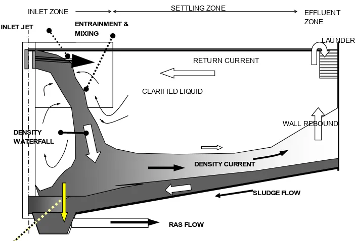
The effects of density differences, between the influent flow and the ambient liquid, in e flow pattern in circular and rectangular clarifiers have been largely studied and ocumented. Density waterfall, entrainment of clarified liquid into the density waterfall increasing the total flow, formation of the bottom density current, rebound at the end wall, recirculation of excess flow, possible short circuiting from the inlet zone to the RAS withdrawal and other associated effects have been identified in field measurements (e.g. Larsen, 1977; Lumley et al., 1988; Samstag et al., 1992; Deininger et al., 1996), as well as in hydraulic model tests (e.g. McCorquodale, 1976, 1977, 1987; McCorquodale et al., 1991; Zhou and McCorquodale, 1992a; Zhou et al., 1992, 1994; van Marle and Kranenburg, 1994; Moursi et al., 1995; Baumer et al., 1996, Krebs et al., 1998 ), and numerical models (e.g. Krebs, 1991; McCorquodale et al., 1991; Zhou and McCorquodale, 1992a, 1992b; Zhou et al., 1992, 1994; Lyn et al., 1992; Krebs et al., 1996). Figure 2.2 shows some of the density associated effects in circular clarifiers. th
INLET ZONE
ENTRAINMENT & MIXING
SETTLING ZONE
EFFLUENT ZONE
RETURN CURRENT
DENSITY CURRENT DENSITY
WATERFALL
SLUDGE FLOW
RAS FLOW
POSSIBLE SHORT CIRCUITING
CLARIFIED LIQUID
LAUNDER
WALL REBOUND
INLET JET
Figure 2.2 Flow Processes in a Circular Clarifier (after McCorquodale, 2004)
2.2.1.1 Modeling Equations
The hydrodynamic and solids stratification of settling tanks have been successfully described by application of the following governing equations and conservation laws:
a) Continuity equation (conservation of fluid mass).
b) Fluid momentum equations (conservation of momentum).
c) Mass transport equation, including the modeling of the settling behavior of the particles (conservation of particulate mass).
Continuity, momentum and mass transport equations have been used in all 2D and 3D models to describe the flow pattern in clarifiers. Few modifications have been introduced in these equations since the original work of Larsen (1977), except in the treatment of the settling velocities [major modifications in the differential equations are presented in the work of Chebbo et al. (1998) and Wells and LaLiberte (1998a)]. On the other hand, different turbulence models have been proposed and used with different levels of success (see section 2.2.3, turbulence models), and few models have included energy considerations (see section 2.2.6, temperature effects).
The following conservation equations can be used to describe two-dimensional, unsteady, turbulent, and density stratified flow in a settling tank using either rectangular or cylindrical co-ordinates (Ekama et al., 1997; McCorquodale, 2004):
Continuity Equation:
0 = y v r + u rm ∂ m
……….. …
r ∂
∂ ∂
(2.1)
Conservation of Momentum in the Radial Direction (r or x):
S + ) y u r ( y r 1 + ) r u r ( r r 1 + r p 1 = y u v + r u u + t u u t m m t m m ∂ ∂ ∂ ∂ ∂ ∂ ∂ ∂ ∂ ∂ − ∂ ∂ ∂ ∂ ∂ ∂ ν ν
ρ … (2.2)
onserv
C ation of Momentum in the Vertical Direction (y):
S + g + ) y v r ( y r 1 + ) r v r ( r r 1 + y p 1 = y v v + r v u + t v v r t m m t m m ρ ρ ρ ν ν ρ − ∂ ∂ ∂ ∂ ∂ ∂ ∂ ∂ ∂ ∂ − ∂ ∂ ∂ ∂ ∂ ∂ …
……… (2.3)
where, … um r 2 ) v r ( r y r 1 + ) u r ( r r r 1 =
) y v r ( y r 1 + ) y u r ( r r 1 =
Sv m m t m m t ∂ ∂ ∂ ∂ ∂ ∂ ∂ ∂ ν
ν ………. (2.5)
is ravitational acceleration in the vertical direction and
in Equations 2.1 to 2.5; m = 1 yields the Cylindrical coordinates, and m = 0 with r = x gives the Cartesian coordinates. The variables u and v are temporal mean velocity components in the r (x) and y directions respectively; p is the general pressure less the hydrostatic pressure at reference density ρr; ρ the fluid density; g is the component of
g νt is eddy viscosity. Equations 2.2
ed
with the inclusion of a density gradients term (
and 2.3 are derived from the Navier- Stokes equations for incompressible fluids, extend
ρ ρ
ρ r
g − ) for the simulation of buoyancy
ffects. e
Conservation of Particulate Mass (Solids Transport) or Concentration Equation:
X) V r + y X r ( y r 1 + ) r X r ( r r 1 = y X v + r X u + t X s m sy m m sr m m ∂ ∂ ∂ ∂ ∂ ∂ ∂ ∂ ∂ ∂ ∂
where X is
∂ ∂
∂
ν
ν ….. (2.6)
concentration of SS; νsr is the eddy diffusivity of suspended solids in the r-(x)
direction; νsy
transport, the sedim
is eddy diffusivity of suspended solids in the y-direction; and Vsis particle settling velocity. By using the Reynolds analogy between mass transport and momentum ent eddy diffusivity can be related to the eddy viscosity νt by the
formula (Zhou and McCorquodale, 1992a; Ekama et al., 1997):
σ ν
sr
= ………. (2.7)
σ ν ν
sy sy
where
t
= ……… (2.8)
σsr and σsy are the Schmidt numbers in the r-(x) direction and the y-direction
respectively. Typical values of the Schmidt number are in the range 0.5 to 1.3 (e.g. Celik and Rodi, 1988; Adams and Rodi, 1990; Zhou and McCorquodale, 1992a, 1992b; Szalai et al., 1994; Krebs et al., 1996; Lakehal et al., 1999).
Using the single-phase flow assumption (which implies that the volume occupied by the solids is negligible), the equations described above can be considered as the theoretical model to represent the major physical processes of solids movement (McCorquodale, 2004). Equations 2.2 and 2.3 (momentum) and Equation 2.6 (mass transfer equation) can be described as a combination of an unsteady term (variation of the property with respect to time), two advective transport terms (describing the fluid-mass transfer process due to convection or flow movement in the plane), two terms related to the eddy diffusion
ixing processes due to turbulent diffusion in two directions) and a source term (which
f the particle settling process. Moreover, source
d diffusion terms are increased to 3 to dicate the space variation of the variables. The buoyancy and the particle settling terms (m
usually extends the ‘pure water’ equation for the simulation of ‘dirty water’). For example, Equation 2.3 includes a source term for the simulation of buoyancy effects and Equation 2.6 a term for the simulation o
terms are also used for the simulation of additional physical and biological process, like flocculation or biological decay processes. In addition to the aforementioned terms, the momentum equations include a pressure gradient term as a flow driving force.
In the case of 3D modeling the convection an in
are not affected by the third dimension.
2.2.2 Settling Properties of the Sludge
Settling particles can settle according to four different regimes, basically depending on e concentration and relative tendency of the particle to interact: 1) discrete particle, 2) compression. In PST the settling process dominated by regimes 1) and 2), but in SST the four settling regimes occur at some
gimes.
Models B
bor th
flocculent particles, 2) hindered or zone, and 4) is
locations and times. A description of the four classes is presented elsewhere (e.g. Takacs et al, 1991; Ekama et al., 1997; Tchobanoglous et al., 2003) and won’t be repeated here. This review focuses on the equations that have been previously presented to model one or more of the four re
ased on Discrete Particles Settling
The settling of discrete particles, assuming no interaction with the neigh ing particles, can be found by means of the classic laws of sedimentation of Newton and Stokes. Equating Newton’s law for drag force to the gravitational force moving the particle, we get Equation 2.9.
p l
l p
d g
sp= 4 (ρ −ρ ) ………
D C V
ρ
3 .. (2.9)
primary particle;
where Vsp is the terminal settling velocity of the CD is the drag oefficient; g is the acceleration due to gravity; ρp and ρl are the particle and liquid icient is a nction of the Reynolds number (NR) and the particle shape. For settling particles NRis c
density respectively; and dp is the diameter of the particle. The drag coeff fu
defined as:
ν
R
N = ……… (2.10)
In Laminar flow (N p d Vsp