Vol. 5, No. 1, 2015, pp.44-68 ISSN: 2146-4138
www.econjournals.com
44
Economic Crises and the Substitution of Fiscal Policy by Monetary Policy
Ioannis N. Kallianiotis1 Economics/Finance Department, The Arthur J. Kania School of Management, University of Scranton, Scranton, PA 18510-4602, USA.
Tel. (570) 941-7577, Fax (570) 941-4825 E-Mail: ioannis.kallianiotis@scranton.edu
ABSTRACT: The paper discusses the latest economic crisis and the public policies used to mitigate the recession and improve the economic growth. The current target rate (monetary policy) is closed to zero since December 2008 with a new experimental policy (“quantitative easing”) to stimulate investment, growth, and employment. The abandonment of the fiscal policy and the current U.S. tax system, which reduces the disposable income and makes savings negative (dissaving or borrowing) has contributed to this slow growth of output and persistent unemployment. This policy has increased the debt of individuals and the low taxes on businesses have magnified the budget deficits and the national debt. Individuals are borrowing the present value of their uncertain future wealth to satisfy their current consumption and their high debt and low income raise the risk and this high risk premium increases the interest rate on uncollateralized loans, especially on credit cards. The U.S. government has to increase corporate taxes, which will lower the national debt; but at the same time, it has to reduce government expenditures (mostly, military expenditures and national defense), curbing inefficiencies, corruption, and increasing public investment (infrastructures). The public policies must be mixed policies (fiscal and monetary) to improve growth and employment first and then to reduce inflation and interest rates. The current one-sided monetary policy and the tax system need to be changed and become optimal, which are essential to improve social welfare, fairness, equity, justice, and to benefit the neglected middle class (the 90% of the population) in the country. This middle class works and pays just taxes and interest (redistribution of its wealth to government and banks), due to its low disposable income, high unemployment, and unfavorable monetary policy. Impoverishing the middle class will deteriorate the entire state of our socio-economic system and it might threaten the existence of the nation.
Keywords: Estimation; Time-Series Models; Consumption and Saving; Taxation; Government Expenditures; Interest Rates; Monetary Policy; Fiscal Policy
JEL Classifications: C13; C22; E21; E43; E52; E62; H20; H50
1. Introduction: The Incitement and Preservation of Economic Crises
In August 2007, a financial crisis began in the U.S. and spread very fast to European and Asian financial markets. By September 2008, this had become a global credit crisis2 and a year later (Fall of 2009) had winded to a global economic crisis with the burdens of the Euro-zone sovereign debt crisis. The seeds of this first economic crisis had been sown with the deregulation of the commercial and investment banking sectors in the 1980s and 1990s and with their new “innovations”. Then, the enormous liquidity, the high debts, the financial and real estate bubbles,3 the bank lending
1
I would like to acknowledge the assistance provided by Jon C. Beckley, Angela J. Parry, and Janice Mecadon. Financial support (professional travel expenses, submission fees, etc.) was provided by the Faculty Travel Funds, Henry George Fund, and FRAP Funds. The usual disclaimer applies. Then, all remaining errors are mine.
2
These were the first negative results of this planned anti-social and anti-national idea of globalization (the destruction of the sovereign nation and its indigenous value system).
3
45 and the securitization practices, created a mountain of risky debts that could not be serviced, when the value of these assets (real and financial) collapsed. These are the results of any exaggeration and lack of control in our societies, but this is the reason that we have governments, regulatory authorities, and central banks to prevent these catastrophic outcomes that affect negatively and disrupt the lives of the citizens of the nation. The questions are, here: What is their national objective? Why they did not act? Who is restricting their power?
The complexity of the nation and its obligations towards the “allies” and the citizens have increased enormously the government spending. These expenditures have to be covered by taxes (government revenue) and borrowing (government securities). The latest consumption had surpassed any previous levels. Individuals were spending a huge proportion of their life wealth by borrowing the present value of their expected future income. The word “saving” was not part of the American vocabulary anymore. Banks, as profit maximizers, were offering without any serious restrictions the amount of money that individuals wanted to borrow by just increasing the risk-premium for a highly indebted customer. As a result of this inconsistent practice individuals ended up with loans, which were exceed their life-cycle income and their interest payment had become an unbearable expense. Banks with their huge risk premiums and their collateral on loans are always winners because even during a financial crisis, we bail them out. The same actions were followed by many nations and their inefficient treasury department; so their debts and deficits have reached the colossal level that are very difficult to be paid back without any unbearable austerities imposed on the citizens or without a general privatizations (sell offs) of the state own enterprises.4 What an illusion that nations were living the last thirty years!
So far all the benefits have gone to the unregulated banks and their executives, which have made huge profits and bonuses from interest income and are intimidating and extorting individuals (with foreclosures) and nations (with sell offs of their SOEs) that have difficulties to pay off their loans. In periods of economic crises, like the 2007-2014, governments (taxpayers) bailed out these failing banks. With this irrational behavior of people and the corruption of governments, banks are ruling them; the socio-politico-economic system (the free market) is at the edge of a steep cliff, which limited the hope for the future from young people. The current crisis is the first in the 21st century and unique in our history; thus, this could not have occurred by chance. Responsible for any of our problems must be the controlled politicians that did not had the power to regulate the corrupted markets and institutions and the uninformed people (voters), who did not prevent the latest systemic crisis by voting out from the government these ineffective politicians.
Unfortunately, the U.S. economy had been characterized for many years with balance of payments imbalances (trade account deficits). But, large current account surpluses realized by Japan in the 1980s and by China in the 1990s and 2000s and were denominated in American dollars, which were recycled back to the U.S. by buying U.S. government and private firms financial assets (debt instruments). These phenomena allowed the U.S. to continue with its twin deficits (trade account5 and budget deficit or national debt6). Also, the low price of Asian products kept inflation low,7 but unemployment high,8 in the U.S.; and because of this low inflation (by construction), a reduced inflation premium and a quantitative easing by the Fed,9 the interest rate stayed low (it was kept closed to zero to enhance the value of the financial assets). With this low cost of capital, consumers were encouraged to increase their indebtedness. Also, this low interest rate generated bubbles in many assets (real, financial, and precious metals). When these bubbles started to burst, the losses of wealth were huge, following by declines in growth and employment in the U.S. and in August 2007 an international financial crisis began and destroyed the Euro-zone economies because of their enormous debts and other socio-political problems that the EU and Euro-zone governments did not expect and
4
See, Kallianiotis (2013).
5
See, BEA, U.S. Department of Commerce, http://www.bea.gov/international/index.htm
6
See, Treasury Direct, http://www.treasurydirect.gov/govt/reports/pd/mspd/2012/2012.htm
7
The U.S. has changed the calculation of CPI twice, first in 1980 and then, in 1990. Methodological shifts in government reporting have depressed reported inflation. For example, the SGS reports an inflation for July 2014 of 10%. See, http://www.shadowstats.com/alternate_data/inflation-charts
8
According to SGS, the unemployment rate in the U.S. with August 2014 was 23.2%. See,
http://www.shadowstats.com/
9
46 did not prevent them, due to their indifference, corruption, common currency, and their control from … Brussels (Germany).10
Further, nations, due to their enormous public expenditures and borrowing have accumulated huge debts and their government revenues are relatively low because of the lesser taxes,11 due to exemptions and deductions that corporations have from the Internal Revenue Code,12 and their unethical practices of tax-avoidance, tax-evasion, and tax-inversion.13 Also, wealthy people are paying less taxes compared to the middle class, which is paying more, lately.14 Consequently, nations pay a lot of interest on these debts (loans), which is in a huge proportion of the total government spending. The U.S. debt exceeded $17.909 trillion and the interest paid in 2013, was $415.7 billion. In 2011, the interest payment was $454.4 billion and in fiscal year 2005, it was $352.4 billion. The reduction in interest rates has decreased the interest cost for the government and for individuals (with refinancing) of the country.15
All city-nations from the ancient times16 had some type of taxation17 because they needed revenue to provide public goods and services and government buildings. Also, for the construction of roads, parks, and schools, to provide police services and the national defense against the foreign invaders. Of course, an efficient management of these tax revenues is important to keep taxes low, growth high and unemployment closed to zero; also, to prevent recessions and keep deficits and
10
Germany had caused two military wars in Europe (WW I from July 28, 1914 to November 11, 1918 and WW II from September 1, 1939 to August 15, 1945) and a third economic war (from 2009-present). What is wrong with European nations that they cannot isolate Germany? Who is behind Germany? What is Germany’s historic role?
11
Taxes always had a high social cost and no one was in favor of high taxes, as we see, today, in the Euro-zone. Also, during the Turkish occupation of South-east Europe (Ottoman Empire, 15th to 19th century). In ancient times, the city of Karystos (Euboea) left the Common of Athens and went with Sparta to avoid the repression and high taxes imposed by Athens to its union members. In 1776, the resentment of the American colonies over U.K. taxes sparked the American Revolution. In 1980, President Reagan was elected president on a platform of large cuts in taxes (Reaganomics), but he did the opposite and became the consignee of deregulation. In 1992, President Clinton was elected in part because president George Bush had broken his 1988 promise, “Read my lips: No new taxes”. But, Bill Clinton raised taxes and generated a budget surplus and a negative saving rate for the households. President George W. Bush promised a tax cut, and he deliver it. The current President, Barack Obama, increased taxes for the high income individuals.
12
Actually, corporations and wealthy people are paying relatively less taxes compared to the middle class and their tax evasion is very high, too. See, Kallianiotis (2014a). Also, Google faces a fight in France over its tax bill. (The Wall Street Journal, October 9, 2014, pp. A1 and A14).
13
The Treasury tries to tighten tax rules to deter U.S. firms from moving their headquarters overseas and slow a wave of so-called corporate inversions that reduce federal government revenues. (The Wall Street Journal, September 23, 2014, pp. A1 and A2).
14
In 1960, the average tax rate (ATR) for the Top 0.1% was 51%, for the Top 1% it was 43%, and for the Middle 20% it was 14%. In 2013, the average tax rate for the Top 0.1% and the Top 1% was 31% and for the Middle 20% it was 19%. (Source: Economic Report of the President 2013, Figure 1-7).
15
See, Bloomberg.com, October 4, 2012. http://www.bloomberg.com/news/2012-10-04/u-s-interest-cost-falls-to-lowest-since-2005-as-debt-soars-1-.html. Also, https://www.treasurydirect.gov/govt/reports/ir/ir_expense.htm. Actually, the interest saving for individuals is not high because there is transaction cost and the bank increases the maturity of the new loan of refinancing. For example: L$50,000, n3years, i7%, the total interest cost is I$5,578.77; by refinancing the same loan with an i4% and a transaction cost of CT$500 and a new
maturity of n5years, the total cost (interest plus transaction) will be: I$5,249.57plus CT $500 = $5,749.57,
which gives a negative saving (loss) of S$170.8. Of course, there is significant saving only if the maturity stays the same (n3years). Then, I$3,143.17plus CT$500=$3,643.17, with a saving of S$1,935.60.
16
In our society, today, we have three taxes. First, income taxes for these people that have an income; then,
lottery tickets, for the people, who have no income (the poor); and lastly, casinos, for those who have no brain (the poor in mind).
17
47 national debts relatively small.18 From 2005 to 2013, Federal taxes have increased by 47.02% (4.7% p.a.). In 2004, individuals were paying (as the Table B-81 shows): 43% + 39% +8% = 90% and corporations: 10% and in 2013 (Table B-80), individuals were paying: 47%+34%+8%=89% and corporations: 11% from the total federal government receipts. These figures reveal the unfairness of our current tax system. The government spending in ten years (2004-2013) has increased by 63.87% (6.4% p.a.). The spending of the U.S. Federal Government in 2004 generated a budget deficit of $412 billion and in 2013 of $992 billion.19 An exaggerated increase in individuals’ taxes, beyond the optimal level (the point of maximization of the social welfare, Graph 1), can increase the budget deficit instead of decreasing it, as it presented, here:
T Y S andC AD Q u Y BD
t D , ,
Then,
T Y S C Y andu recession T BD
t D 0,
where, t = tax rate, T = taxes, YD = disposable income, S = saving, C = consumption, AD = aggregate demand, Q = output, u = unemployment, Y = income, BD = budget deficit, = increase, = decrease, and = drastic increase.
The national defense is the defense of the nation from “foreign aggressors” and it is one of the most expensive from all public goods. In 2004, the U.S. federal government spent a total of $456 billion on national defense, more than $1,500 per person. In 2010, the spending was $683.7 billion,20 which was more than $2,220 per person, without foreign aggression. The total government revenue (including federal, state, and local) as a percentage of total income has grown substantially over the past century. In 1902, the government collected 7% of total income; in recent years, government has received 30% of the income.21 Also, state and local governments collect about 40% of all taxes paid. The revenues and spending of the state and local governments in 2002 exhibit a deficit of $50 billion and in 2010 it fell a little to $41 billion.22
Unfortunately, U.S. debt23 had surpassed 122% of GDP and deficits had tended to be around 9% to 11% during the latest financial crisis. This was partly due to industry rescue plans (bailouts), stimulus plans, and economic stabilizers (i.e., unemployment benefits, etc.). The chronic deficits come from uniquely American characteristics (market oriented economy), which in large part has been caused by policies of tax reductions, especially for the upper income groups and businesses since 1980s. Taxes are going up for everyone with the new fiscal cliff deal on January 1, 2013.24 Also, it is an increase in spending for Medicare (prescription drugs) and for the wars (in Iraq, Afghanistan, Syria, Ukraine, Levant, etc.). America’s problems, so far, were limited, due to relatively good economic growth because of demographic growth (massive immigration and relatively high fertility rates) and because of the dollar’s preeminent role as the international reserve currency since 1944.25 The Fed provides the dollars (Fed’s liabilities) that are used to pay for the nation’s deficits by buying the government debt instruments (U.S. Treasury liabilities). A fragile world based on recycling of liabilities without generating real economic growth.26
18
See, Kallianiotis (2015) and Economic Report of the President 2005, Table B-81and 2013, Table B-80. http://www.whitehouse.gov/sites/default/files/docs/full_2014_economic_report_of_the_president.pdf 19
See, Kallianiotis (2015) and Economic Report of the President 2005, Table B-81 and 2013, Table B-80. 20
See, http://en.wikipedia.org/wiki/Military_budget_of_the_United_States
21
See, Historical Statistics of the United States; Bureau of Economic Analysis.
22
See, Kallianiotis (2015) and Economic Report of the President 2005 and 2013, Table B-86. 23
Taking into consideration Social Security and the other entitlements, the national debt is 870.45% of the GDP. Examples of entitlement programs at the federal level in the United States include Social Security, Medicare and
Medicaid, most Veterans' Administration programs, federal employee and military retirement plans,
unemployment compensation, food stamps, and agricultural price support programs.
24
See, http://economy.money.cnn.com/2013/01/02/taxes-fiscal-cliff/. To avoid the fiscal cliff, President Obama signed the American Taxpayer Relief Act of 2012 (ATRA) on January 2, 2013. While payroll taxes, income taxes, capital gains taxes, and dividend taxes all increased for the highest earners, for most taxpayers’ increases were modest. See, McGranahan and Nohel (2014, Figure 1).
25
See, Kallianiotis (2014b and c).
26
48 The literature on this subject is extensive. Ramsey (1927) and Mirrlees and Diamond (1971a and b) discuss the optimal tax policy. Giannoni and Woodford (2002) offer general conditions under which optimal policy can be represented by a “super-inertial” interest rate or by a pure “targeting rule”. Faia and Monacelli (2007) use a welfare-maximizing interest rate rule and found that monetary policy should respond to increases in asset prices by lowering interest rates, but when monetary policy responds strongly to inflation, the marginal welfare gain of responding to asset prices vanishes. Allen and Gale (2009) present with a unique way the financial crises. Mankiw, Weinzierl, and Yagan (2009) explore the interplay between tax theory and tax policy. Wessel (2009) discusses step by step the latest financial crisis and the role of the U.S. Treasury and of the Fed as the fourth branch of government. Krugman (2013) recommends high taxes for the rich. Given (2013) gives four principles of optimal taxation to facilitate prosperity. Eiteman, Stonehill, and Moffett (2013) analyze the factors that caused this continuing global financial crisis. McGranahan and Nohel (2014) examine the reaction of corporations and individuals in an effort to minimize the tax burden of the ATRA of 2012. Saving (2014) says that the deficit has declined, but the debt is going up and it will fall on the future generations. Kallianiotis (2014a) discusses the enormous debts, the current tax system, and regards as the ultimate objective of a nation the social welfare of its citizens. Kallianiotis (2014b) shows that reduction in taxes and increase in government spending are necessary policies for the U.S. and the Euro-zone to improve currently their economies. Heathcote, Storesletten, and Violante (2014) develop a model and discuss the parameters that influence the degree of optimal tax progressivity. Kallianiotis (2014d) discusses the current interest rate system and compares it with the optimal interest rate, which can improve social welfare.
2. A Theoretical Model
In the past, taxes were much lower for individuals and thus, the disposable income was higher. Also, saving was a virtue that was a small complement of the other values of our socio-economic system and this money was deposited to the financial institutions (intermediation). Historically, consumption was always a function of income, which is a risk-free prudent human behavior,
) ( t t f Y
C (1)
or better, current consumption must be a function of the previous period (earned) income, )
( 1
t
t f Y
C (1’)
where, Ct= consumption and Yt = income.
But, the last years of delusion and pseudo-prosperity, the current consumption has become a function of the present value of the expected life wealth. But, mostly this wealth belongs to the rich people and does not have any wealth effect on the nation’s consumption and on our aggregate demand, production, growth, and employment. Only, the rich are becoming richer without any extra spending because they have already satisfied all their needs (actually, their wants) and the middle class becomes poorer because of its debt and the economy has no social benefits from this wealth effect of the wealthy.27 Thus,
)] ( [ t t f EW
C (2)
where, E(Wt)= present value of the expected wealth in period t.
The objective of the Fed is stabilization of output (maximum employment) and prices (inflation target 2% or less per annum) by pursuing its monetary policy. Central bank’s behavior (reaction to inflation and output-employment) can be presented with an interest rate reaction function, eq. (3), as follows:
)
(
)
(
)
(
)
1
(
* *1
N t t u t t t
t FF
FF
i
r
u
u
i
t
t
(3)27
Americans’ wealth hit a record $81.8 trillion in the first quarter of 2014 amid a rise in home values and stock prices. See, The Wall Street Journal, June 6, 2014, pp. A1 and A2. But, the distribution of this wealth is completely unfair; about 50 million Americans live below the poverty line and a record 47 million of them receive food stamps. The federal government defines the poverty line as a family of four earning $23,550. See,
49 where,
t
FF
i
= the target federal funds rate,
t= the rate of inflation as measured by the GDP deflator,*
t
= the desired rate of inflation,28 * tr = the assumed equilibrium real interest rate, ut= the unemployment rate, N
t
u = the natural level of unemployment, and
= the weight put on the past federal funds rate setting.We can run a regression of eq. (3), which can be eq. (4). The target interest rate will follow the changes in inflation and unemployment based on the coefficients estimated in eq. (4). This interest rate measured by the interest rate reaction function must be the target federal funds rate:
t GAP t GAP t t FF
FF
i
u
u
i
t
t
0
1 1
2
3
4 1
(4)where,
u
GAPt
u
t
u
tN.Using monthly data for the U.S. economy (1954:M08-2014:07), we have:
720 , 396 . 1 , 797 . 814 , 8 , 502 . 0 , 980 . 0 ) 098 . 0 ( ) 098 . 0 ( ) 005 . 0 ( ) 006 . 0 ( ) 041 . 0 ( 547 . 0 577 . 0 016 . 0 984 . 0 080 . 0 2 1 * * * * * * * * * * * * * * 1 N W D F SER R u u i i GAP t GAP t t FF
FFt t
The size of the partial adjustment, coefficient 1, which is 0.984*** provides direct evidence that the observed degree of persistence in federal funds rates is greater than the one that can be attributed to systematic policy responses to persistent inflation and unemployment (output) fluctuations. The coefficients of regression show that the federal funds rate must respond significantly
to an increase in inflation (
20.016***), but less aggressively to induce an increase in real rates and atightening monetary policy. The federal funds rate must respond sufficiently aggressively to an
increase in unemployment (30.577***) to induce a reduction in interest rate and an effective easing
monetary policy.
Further, the Taylor rule is a specific case of eq. (3); it puts 0 and by substituting the logarithm of GDP with the unemployment rate, we get the following equation:
)
(
)
(
* * N t t u t t t tFF
r
u
u
i
t
(5)Taylor (1993) proposed an
0
.
5
and
u
0
.
5
.29
The rule “recommends” a high interest rate (a “tight” monetary policy) when inflation is above its target, in order to reduce inflationary pressure and a low interest rate (“easy” monetary policy) when the unemployment rate is above its natural level to stimulate production, output, and employment.30
Lately, the relatively lower interest rates have reduced the pressure that debt service places on the budget. It obvious that interest rates will increase as the economy will improve and the interest payment on debt will augment the budget deficit. Higher debt is necessary in some cases (i.e., recessions), where the government relies on public debt to finance infrastructure (roads, bridges, and
28
The Fed ultimately stated explicitly that its target was a 2% per year increase in the raw personal consumption expenditures deflator. See, Williamson (2014, p. 112). Here, we forecast the (desired) inflation, as follows:
772 , 007 . 2 , 987 . 169 , 507 . 3 , 307 . 0 ) 035 . 0 ( ) 036 . 0 ( ) 176 . 0 ( 172 . 0 442 . 0 382 . 1 2 2 * * * 1 * * * * * * * N W D F SER R t t t e
t
29
Also, there is a Phillips curve in our economy: t te(ututN)t, which gives the following regression:
719 , 073 . 2 , 258 . 3 , 373 . 0 ) 066 . 0 ( ) 039 . 0 ( ) 4 ( 160 . 0 064 . 1 2 * * * * * N W D SER R ut e t t 30
If the economy is in a recession (with high unemployment, i.e., 6.5%), we must have a target interest rate:
% 75 . 1 %) 4 % 5 . 6 ( 5 . 0 %) 2 % 2 ( 5 . 0 % 1 %
2
FF
i . This must be the federal funds rate today (September
50 other public investments) and to promote economic growth and employment. These public capital contribute to private sector investment, productivity, output, and employment. It improves the social welfare, as it is shown below.
Taxes can be referred as the sums of a variety of different components of direct (i.e., income taxes, etc.) and indirect taxes (i.e., sale tax, etc.),31 with their objective to generate the necessary government revenue and to improve the distribution of wealth among people and businesses.
t t t t t t
t SG LG P M SS S PPC
FG
t
T
T
T
T
T
T
T
T
&
(6)where, Tt = total taxes,
T
FGt= federal government tax,T
SGt= state government tax,T
LGt= localgovernment tax,
T
Pt= property tax,T
M&SSt= Medicare and social security “tax” contribution,T
St=sale tax, and
T
PPCt= private pension contribution.The demand for loans (Ldt ) by individuals, due to their insufficient income, can be written as functions of the following variables:
0 , 0 , 0 , 0 , 0 , 0 ) , , , , , ( f f f f f f i T C u Y f L i T C u Y t t t t t t d t (7)
where, Lt = loans,
u
t= unemployment rate,i
t = loans’ rate, and
t = uncertainty.The supply of loans (Lst ) by the banks is determined by the same variables as the demand for loans, but the effects are different because the objective, here, is banks’ profitability.
0 , 0 , 0 , 0 , 0 , 0 ) , , , , , ( f f f f f f i T C u Y f L i T C u Y t t t t t t s t (7’)
The consumption of individuals can be functions of the variables,
0 , 0 , 0 , 0 , 0 , 0 , 0 , 0 , 0 , 0 , 0 ] , , , , , , , ), ( , , [ ) ( f f f f f f f f f f f t T I i DP L W E u Y f C MCI t T I i DP L W E u Y t MCI t t t t t t t t t t (8)
where, t= inflation or prices (CPI), DPt = debt payment (of annuities), It = interest payment, and
MCI
t
= tax rate on middle class individuals.The tax (government revenue) function can be written,
0 , 0 , 0 , 0 , 0 , 0 , 0 , 0 , 0 , 0 , 0 ) , , , , , , , , , , ( ND BD G GS t t t t Y Y Y t t t t t C WI MCI C WI MCI t f f f f f f f f f f f ND BD G GS t t t t Y Y Y f T C WI MCI C WI MCI t t t t t t (9)
where,
Y
MCIt = income of middle class individuals ($30,000-$150,000 per annum),Y
WIt= income ofwealthy individuals (over $150,000 per annum),
Y
Ct= income of corporations (businesses),t
MCI
t = tax
rate of middle class individuals,
t
WIt= tax rate of wealthy individuals,t
Ct= tax rate of corporations,t
t
= tariff (import tax), GSt = government subsidies (tax exemptions, tax savings, tax reductions, and bail outs),Gt= government spending, BDt= budget deficit, and NDt= national debt.32
The fiscal policy satisfies the social objectives by using taxes and government spending and public investment. Thus, there must be an optimal tax rate, which is the tax that balances the
31
Taxes are lowering the welfare, due to losses to buyers and sellers from a tax that exceeds the revenue raised by the government, which is the deadweight loss (reduction in consumer and producer surplus). Consequently, our demand for any product or service must be relatively inelastic ( 1) to reduce the deadweight loss; but
this is against us because we will pay high prices and thus, higher cost for our goods and services with inelastic demands. See, Mankiw (2007, p. 166).
32
51 government budget or generates a surplus during periods of growth and generates a deficit during periods of recession. But, in both economic conditions the social welfare is maximized. The bliss point is reached, as it is shown in Graph 1.
Boom: GBtTtGt0
) ,... , (
max Utf utAutB utN
(10)
Recession: GBtTtGt0
where, GBt= government budget, Ut= social welfare function, and utA,utB,...utN= utility of
individual A, B, and N.
The optimal taxation is the one that maximizes the social welfare in the country. The average tax rate (ATR) of corporations (ATRC) must exceed the ATR of individuals (ATRI). When ATRs are high, businesses are moving abroad and individuals work less and the government spends more, hoping to cover these high expenditures, but T<G. Then, ATR must fall, which will affect positively net income, disposable income, consumption, and saving. These increases will raise aggregate demand, production, employment, income and of course, tax revenue. Consequently, T=G and the social welfare will enhance and it will reach its maximum level (U*). This is the point (bliss) where the marginal benefits from the average tax rate reduction will be offset by the marginal cost, due to higher taxes (MBATRRMCHT ). After this optimal level of taxes, the ATR is increasing, disposable income is falling, which affects negatively consumption, saving, aggregate demand, production, employment, and income. Now, T>G, but this redistribution of wealth from citizens to government reduces the social welfare and after a level, it can become negative (Graph 1), as it is in some Euro-zone nations, after the Troika’s austerities.
Lastly, to see the effects of monetary and fiscal policy on our economy, we can use a vector auto-regression (VAR) with dependent variables
u
t and
t and independent ones the policy tools, as follows: t t t t t FF FF t t t t t t t t t t FF FF t t t t t g g t t i i u u g g t t i i u u u t t t t 2 1 20 29 1 28 27 26 25 2 24 1 23 2 22 1 21 20 1 1 20 19 1 18 17 16 15 2 14 1 13 2 12 1 11 10 1 1 (11)where, ttlnTt= tax or government revenue and gtlnGt= government spending. The estimation of the above VAR, eq. (11), will tell us the effectiveness of the two public policies, monetary and fiscal.
3. Empirical Results
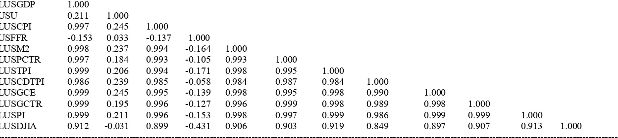
It is important to test the above equations by applying data from the U.S. economy. The data, taken from economagic.com, Yahoo.com, and Bloomberg.com are monthly from 1959:01 to 2014:03. They comprise, consumption (USPCE), income (USPI), money supply (M2), Dow Jones Industrial Average (USDJIA) (price of stocks), wealth (USW=M2+USDJIA), U.S. wages and salaries (USWS), corporate profit (USCYP), U.S. personal current taxes (USPCTR) (taxes on middle class), taxes on corporations (USTPI) (taxes on production and imports), custom duties on production and imports (USCDTPI) (tariffs), government subsidies (USGS), government current (spending) expenditures (USGCE), budget deficit (USBD), national debt (USND), loans or consumer credit outstanding (USCCO), unemployment rate (USU), taxes or U.S. government current tax receipts (USGCTR), federal funds rate (USFFR), prime rate (USPR), interest rate or corporate bonds rate (Baa), LIBOR 3-month rate (LIBOR3M), 3-3-monthe U.S. T-Bill rate (STT3M), TED rate for measuring the risk (=LIBOR3M-STT3M), gold prices (GOLD) for measuring again uncertainty, consumer price index (USCPI), U.S. gross domestic product (USGDP), and U.S. personal income (USPI).
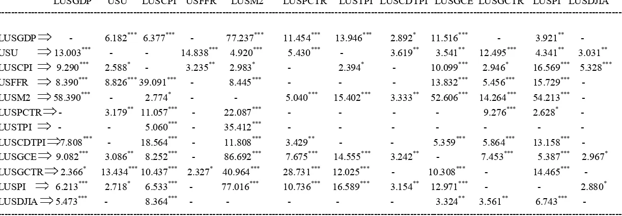
First, the correlation coefficients and a Granger causality test between most of these variables are presented in Tables 1 and 2. First, the effect of monetary policy is examined. The federal funds cause gross domestic product (-8.390***),33 cause unemployment (+8.826***), cause inflation
33
52 39.091***),34 cause money supply (-8.445***) liquidity effect, cause government current expenditures (-13.832***), cause current tax receipts (-5.456***), and cause personal income (-15.729***). Then, the money supply causes GDP (+58.390***), causes inflation (+2.774*),35 causes personal taxes (+5.040***), causes taxes on production and imports (+15.402***), causes custom duties (+3.333***), causes government current expenditures (+52.606***), causes current tax receipts (+14.264***), and it causes personal income (+54.213***), too. Now, the effect of fiscal policy shows the following results. Taxes cause GDP (+2.366*), cause unemployment (+13.434***), cause inflation (+10.437***), cause federal funds (-2.327*), cause money supply (+40.964***), cause personal current taxes (+28.731***), cause taxes on production and imports (+12.025***), cause government current expenditures (+10.308***), and cause personal income (+14.465***). Government expenditures cause GDP (+9.082***), cause unemployment (+3.086**), cause inflation (+8.252***), cause money supply (+86.692***),36 cause personal current taxes (+7.675***), cause taxes on production and income (+14.555***), cause custom duties (+3.242**), cause government current tax receipts (+7.453***), cause personal income (+5.387***), and cause also DJIA (+2.967*).
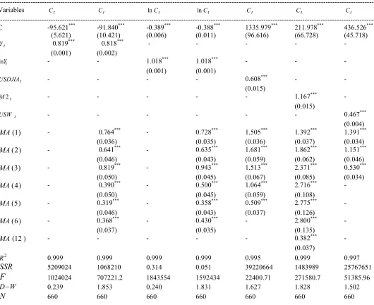
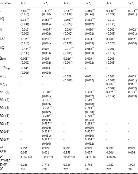
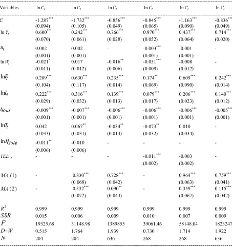
Then, Table 3 shows the estimates of consumption by using eqs. (1) and (2). Personal income has a significant effect on consumption; stock prices, money supply (liquidity), and wealth have all significant positive effect on consumption, too. Table 4 gives the estimation of eq. (7’). Loans (consumer credit outstanding) are affected positively by income and consumption; negatively by unemployment, taxes, and risk. Table 5 presents the estimate of consumption of eq. (8). Consumption is affected positively by income, prices, and loans; it is affected negatively by unemployment, wealth, interest rate, taxes, and risk. An increase in wealth reduces consumption because this wealth belongs to the rich people and already they consume at their maximum level; but, the distribution of wealth is a problem, the wealth of the poor people is falling and for this reason consumption is falling, too. Prices are going up and consumption is increasing (inelastic demand for consumer’s goods and services).
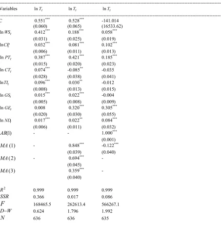
Further, Table 6 gives the results from eq. (9). Wages & salaries (income of middle class), corporate profit, personal taxes (on middle class), tariffs on imports, government subsidies, government spending, and national debt have a significant positive effect on government revenue (taxes). Corporate taxes have a negative effect on government revenue. Consequently, tax revenue can grow with an increase in money supply (inflationary finance), an increase in corporate profit, an imposition of tariffs, an increase in the market value of financial assets (DJIA), and a reduction in interest rate. There is no need to raise taxes on individuals because the social welfare is falling. Also, the government spending has to be moderate, efficient, and at the level that satisfies domestic public services, public goods, and public capital investment.
34
With this zero federal funds rate, we will have very high inflation. A housewife asked me; how much is the inflation in the U.S.? I sent to her that the official sources say 1.7% and independent researchers ascent it to 10%. Then, she sent to me; the last couple of years the prices in most of the items have been doubled. It is obvious that the laypeople know better than us, the so-called “economists”.
35
The F-Statistic, here, show that this enormous growth in money has a very small effect on inflation. Then, the conclusion can be that prices are not a monetary phenomenon or that the high unemployment (double digit unemployment) keeps the inflation low or that the data on inflation are wrong (underestimated).
36
53
Table 1. Correlation Coefficients
---
LUSGDP USU LUSCPI USFFR LUSM2 LUSPCTR LUSTPI LUSCDTPI LUSGCE LUSGCTR LUSPI LUSDJIA ---
LUSGDP 1.000
USU 0.211 1.000
LUSCPI 0.997 0.245 1.000
USFFR -0.153 0.033 -0.137 1.000
LUSM2 0.998 0.237 0.994 -0.164 1.000
LUSPCTR 0.997 0.184 0.993 -0.105 0.993 1.000
LUSTPI 0.999 0.206 0.994 -0.171 0.998 0.995 1.000
LUSCDTPI 0.986 0.239 0.985 -0.058 0.984 0.987 0.984 1.000
LUSGCE 0.999 0.245 0.995 -0.139 0.998 0.995 0.998 0.990 1.000
LUSGCTR 0.999 0.195 0.996 -0.127 0.996 0.999 0.998 0.989 0.998 1.000
LUSPI 0.999 0.211 0.996 -0.153 0.998 0.997 0.999 0.986 0.999 0.999 1.000
LUSDJIA 0.912 -0.031 0.899 -0.431 0.906 0.903 0.919 0.849 0.897 0.907 0.913 1.000
--- Note: LUSGDP = ln of U.S. gross domestic product, USU= U.S. unemployment rate, LUSCPI = ln of U.S. consumer price index, USFFR = U.S. federal funds rate, LUSM2 = ln of U.S. money supply (M2), LUSPCTR = ln of U.S. personal current taxes (taxes on middle class), LUSTPI = ln of U.S. taxes on production and imports (taxes on corporations), LUSCDTPI = U.S. custom duties on production and imports (tariffs), LUSGCE = ln of U.S. government current expenditures (government spending), LUSGCTR = ln of U.S. government current tax receipts, LUSPI = ln of U.S. personal income, and LUSDJIA = ln of U.S. Dow Jones Industrial Average (price of stocks).
54
Table 2. Granger Causality Test
--- LUSGDP USU LUSCPI USFFR LUSM2 LUSPCTR LUSTPI LUSCDTPI LUSGCE LUSGCTR LUSPI LUSDJIA ---
LUSGDP
- 6.182*** 6.377*** - 77.237*** 11.454*** 13.946*** 2.892* 11.516*** - 3.921** -USU
13.003*** - - 14.838*** 4.920*** 5.430*** - 3.619** 3.541** 12.495*** 4.341** 3.031**LUSCPI
9.290*** 2.588* - 3.235** 2.983* - 2.394* - 10.099*** 2.946* 16.569*** 5.328*** USFFR
8.390*** 8.826*** 39.091*** - 8.445*** - - - 13.832*** 5.456*** 15.729*** -LUSM2
58.390*** - 2.774* - - 5.040*** 15.402*** 3.333** 52.606*** 14.264*** 54.213*** -LUSPCTR
- 3.179** 11.057*** - 22.087*** - - - - 9.276*** 2.628* - LUSTPI
- - 5.060*** - 35.412*** - - - - - - -LUSCDTPI
7.808*** - 18.564*** - 11.808*** 3.429** - - 5.359*** 5.864*** 13.158*** - LUSGCE
9.082*** 3.086** 8.252*** - 86.692*** 7.675*** 14.555*** 3.242** - 7.453*** 5.387*** 2.967*LUSGCTR
2.366* 13.434*** 10.437*** 2.327* 40.964*** 28.731*** 12.025*** - 10.308*** - 14.465*** -LUSPI
6.213*** 2.718* 6.533*** - 77.016*** 10.736*** 16.589*** 3.154** 12.971*** - - 2.880*LUSDJIA
5.473*** - 8.364*** - - - - - 3.324** 3.561** 6.743*** ---- Note:See, Table 1.
= causes, ***= significant at the 1% level, ** = significant at the 5% level, and * = significant at the 10% level.55
Table 3. Estimates of Consumption: Eqs. (1) and (2)
---
Variables Ct Ct lnCt lnCt Ct Ct Ct
--- C -95.621*** -91.840*** -0.389*** -0.388*** 1335.979*** 211.978*** 436.526***
(5.621) (10.421) (0.006) (0.011) (96.616) (66.728) (45.718)
t
Y 0.819*** 0.818*** - - - -
(0.001) (0.002)
t
Y
ln - - 1.018*** 1.018*** - - -
(0.001) (0.001)
t
USDJIA - - - - 0.608*** - -
(0.015)
t
M2 - - - 1.167*** -
(0.015)
t
USW - - - 0.467***
(0.004)
) 1 (
MA - 0.764*** - 0.728*** 1.505*** 1.392*** 1.391***
(0.036) (0.035) (0.036) (0.037) (0.034)
) 2 (
MA - 0.641*** - 0.635*** 1.681*** 1.862*** 1.151***
(0.046) (0.043) (0.059) (0.062) (0.046)
) 3 (
MA - 0.819*** - 0.943*** 1.513*** 2.371*** 0.530***
(0.050) (0.045) (0.067) (0.085) (0.034)
) 4 (
MA - 0.390*** - 0.500*** 1.064*** 2.716*** -
(0.050) (0.045) (0.059) (0.108)
) 5 (
MA - 0.319*** - 0.358*** 0.509*** 2.775*** -
(0.046) (0.043) (0.037) (0.126)
) 6 (
MA - 0.368*** - 0.430*** - 2.800*** -
(0.037) (0.035) (0.135)
) 12 (
MA - - - 0.382*** -
(0.037) 2
R 0.999 0.999 0.999 0.999 0.995 0.999 0.997
SSR 5209024 1068210 0.314 0.051 39220664 1483989 25767651
F
1024024 707221.2 1843554 1592434 22400.71 271580.7 51385.96W
D 0.239 1.853 0.240 1.831 1.627 1.828 1.502
N 660 660 660 660 660 660 660
---
56 The estimation of the VAR, eq. (11), gives the following results:
713 , 847 . 42 , 275 . 3 , 379 . 0 : ; 713 , 379 . 5507 , 180 . 0 , 987 . 0 : ) 011 . 13 ( ) 788 . 12 ( ) 284 . 9 ( ) 194 . 9 ( 714 . 0 248 . 8 235 . 18 089 . 9 ) 247 . 0 ( ) 247 . 0 ( ) 038 . 0 ( ) 038 . 0 ( ) 678 . 0 ( ) 692 . 0 ( ) 099 . 1 ( 260 . 0 641 . 0 073 . 0 331 . 0 641 . 0 272 . 0 692 . 2 ) 717 . 0 ( ) 704 . 0 ( ) 511 . 0 ( ) 506 . 0 ( 780 . 1 475 . 2 273 . 2 980 . 2 ) 014 . 0 ( ) 014 . 0 ( ) 002 . 0 ( ) 002 . 0 ( ) 038 . 0 ( ) 038 . 0 ( ) 061 . 0 ( 075 . 0 068 . 0 001 . 0 003 . 0 050 . 0 013 . 1 199 . 0 2 2 1 1 * * * * * 2 * * 1 * * * 2 1 * * * 1 * * * * * * 1 * * * * * * * * * * * * 2 1 2 1 * * * * * * 1 1 N F SER R N F SER R u g g t t i i u u g g t t i i u u u t t t t FF FF t t t t t t t t t FF FF t t t t t t t t t
The results show that the monetary policy tool (federal funds) have a small positive correlation with unemployment rate (+0.033) and cause unemployment (8.826***). The VAR reveals that the current federal funds have a significant negative effect on unemployment (the zero target rate increases or does not reduce unemployment), but the previous federal funds rate has a significant positive effect on unemployment. Also, federal funds have a negative effect on inflation (-0.137) and cause inflation (39.091***). Then, inflation is creeping even though that we have changed its way of measuring. The regression points a significant positive effect of federal funds on inflation. Taxes have a small positive correlation with unemployment (+0.195) and cause unemployment (13.434***). Thus, during periods of recession, we must reduce taxes. An increase in current taxes has a significant reduction in unemployment, but an increase in last period taxes increase unemployment. Taxes have a high positive correlation with inflation (+0.993) and cause inflation (10.437***). Last period taxes have a significant negative effect on inflation (because disposable income is falling and AD falls). Government spending has a small correlation with unemployment (+0.245) and causes unemployment (3.086**). The regression shows that the current government spending has a positive significant effect on unemployment and last period’s government spending has a significant negative effect on unemployment. The government spending has a high correlation with inflation (+0.995) and causality (8.252***). The regression does not indicate any significant effect of government spending on inflation.
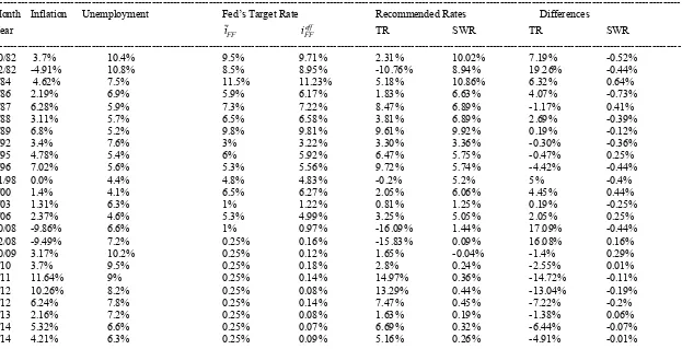
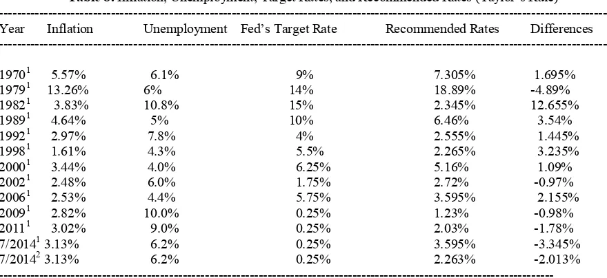
Lastly, by using the Sack-Wieland (SWR) and the Taylor rule (TR), eqs. (4) and (5), we determine the target rate during the periods 1982-2014 and 1970-2014. The results appeared in Tables 7 and 8, where it is obvious that most of the times the Fed’s target rate is above the recommended rate, which is very helpful for the financial market, but not for the other sectors of the economy. In 1979 and lately, after 2009, the Fed’s rate is below the recommended by Taylor’s rule, with its objective to improve the economy that was in a recession and to reduce the double digit unemployment rate; but unfortunately, it has been proved to be ineffective (low growth and high unemployment) and it has created a new bubble in the financial market,37 a devaluation of the dollar, inflation in the economy, negative real return to savers (redistribution of wealth from individuals to banks and speculators), and encouragement of outsourcing (“internal devaluation” to make wages and salaries and the level of economic welfare the same as in developing countries, due to globalization).The economy needs a mixed public policy, fiscal and monetary to recover from this latest unique global (systemic) financial crisis and a necessary protection for the domestic industries from the foreign rivals, reduction in middle class taxes, and regulation of the financial market, institutions, and their “innovative” instruments.
57
Table 4. Estimates of Supply of Loans: Eq. (7’)
---
Variables lnLt lnLt lnLt lnLt lnLt lnLt
--- C 2.892*** 3.437*** 1.463*** 2.660*** 0.140*** 0.124***
(0.113) (0.180) (0.181) (0.146) (0.029) (0.021)
t Y
ln 0.324** 0.363*** 1.098*** 0.382*** -0.012 - (0.140) (0.065) (0.222) (0.062) (0.033)
t
u -0.011*** -0.005** -0.036*** -0.010*** -0.002*** -0.002*** (0.002) (0.002) (0.002) (0.002) (0.001) (0.001)
t C
ln 1.376***
0.857*** 0.977*** 0.874*** 0.060** 0.052*** (0.112) (0.061) (0.178) (0.058) (0.027) (0.009)
t T
ln -0.424*** 0.007 -0.714*** 0.062** -0.001 -
(0.537) (0.033) (0.085) (0.033) (0.014)
t Baa
i 0.008***
0.003 0.026*** 0.003 -0.001 -
(0.002) (0.002) (0.004) (0.002) (0.001)
t Gold P
ln -0.045*** -0.003 - - - -
(0.006) (0.008)
t
TED - - -0.028*** -0.001 -0.002* -0.003***
(0.008) (0.002) (0.001) (0.001)
1
lnLt - - - - 0.962*** 0.961***
(0.009) (0.007) )
1 (
MA - 1.110*** - 1.346*** 0.175*** 0.173***
(0.061) (0.052) (0.059) (0.059)
) 2 (
MA - 1.181*** - 1.589*** - -
(0.079) (0.080)
) 3 (
MA - 1.305*** - 1.784*** - -
(0.092) (0.100)
) 4 (
MA - 1.269*** - 1.702*** - -
(0.094) (0.105)
) 5 (
MA - 0.987*** - 1.283*** - -
(0.094) (0.099)
) 6 (
MA - 0.813*** - 0.927*** - -
(0.081) (0.080)
) 7 (
MA - 0.538*** - 0.524*** - -
(0.060) (0.052)
2
R 0.996 0.999 0.994 0.999 0.999 0.999
SSR
0.089 0.011 0.358 0.017 0.006 0.004F
9104.328 33537.71 7959.708 74711.02 370426.1597468.7
W
D 0.266 1.778 0.185 1.754 1.922 1.923
N
228 228 292 292 292 292---
58
Table 5. Estimates of Consumption: Eq. (8)
---
Variables lnCt lnCt lnCt lnCt lnCt lnCt
--- C -1.287*** -1.732*** -0.856*** -0.845*** -1.163*** -0.836*** (0.094) (0.105) (0.049) (0.065) (0.090) (0.049)
t Y
ln 0.600*** 0.242*** 0.766*** 0.970*** 0.437*** 0.714*** (0.070) (0.061) (0.028) (0.052) (0.064) (0.020)
t
u 0.002 0.002 - -0.003*** -0.001 -
(0.001) (0.001) (0.001) (0.001)
t
W
ln -0.021* 0.017 -0.016** -0.051*** -0.008 -
(0.011) (0.012) (0.006) (0.009) (0.012)
t P
ln 0.289*** 0.630*** 0.235*** 0.174** 0.609*** 0.242*** (0.104) (0.117) (0.014) (0.069) (0.090) (0.014)
t L
ln 0.222*** 0.316*** 0.139*** 0.079*** 0.206*** 0.140*** (0.029) (0.032) (0.013) (0.017) (0.023) (0.012)
t Baa
i -0.009*** -0.007*** -0.006*** -0.006*** -0.006*** -0.005*** (0.001) (0.001) (0.001) (0.001) (0.001) (0.001)
t T
ln 0.042 0.067** -0.034** -0.073** 0.010 -
(0.033) (0.031) (0.014) (0.032) (0.034)
t Gold
P
ln -0.011** -0.010 - - - -
(0.006) (0.006)
t
TED - - - -0.011*** -0.003
-(0.002) (0.002)
) 1 (
MA - 0.830*** 0.728*** - 0.964*** 0.759***
(0.068) (0.042) (0.063) (0.041)
) 2 (
MA - 0.332*** 0.090** - 0.359*** 0.115***
(0.072) (0.043) (0.067) (0.042)
2
R 0.999 0.999 0.999 0.999 0.999 0.999
SSR
0.015 0.006 0.009 0.010 0.007 0.009F
19325.68 31148.98 1389855 39061.46 58148.04 1823247W
D 0.515 1.764 1.939 0.730 1.714 1.922
N
204 204 636 268 268 636---
59
Table 6. Estimates of Taxes (Government Revenue): Eq. (9)
---
Variables lnTt lnTt lnTt
--- C 0.551*** 0.528*** -141.014
(0.060) (0.065) (16533.62)
t WS
ln 0.412*** 0.188*** 0.058*** (0.031) (0.025) (0.019)
t CP
ln 0.032*** 0.081*** 0.102*** (0.006) (0.011) (0.013)
t PT
ln 0.387*** 0.421*** 0.185*** (0.015) (0.020) (0.023)
t CT
ln 0.074*** -0.085** -0.035 (0.028) (0.038) (0.041)
t TI
ln 0.096*** 0.030** -0.012 (0.008) (0.013) (0.015)
t
GS
ln 0.015*** 0.022*** -0.004 (0.005) (0.008) (0.009)
t
GE
ln 0.008 0.320*** 0.305*** (0.020) (0.030) (0.055)
t
ND
ln 0.017*** 0.022** 0.084*** (0.006) (0.011) (0.032) )
1 (
AR - - 1.000***
(0.001) )
1 (
MA - 0.848*** -0.122***
(0.039) (0.040) )
2 (
MA - 0.694*** -
(0.045) )
3 (
MA 0.359*** -
(0.040)
2
R 0.999 0.999 0.999
SSR 0.366 0.017 0.086
F
168465.5 262613.4 566267.1W
D 0.624 1.796 1.992
N
636 636 635---
Note: See, Tables 1 and 2. WSt= wages and salaries, CPt= corporate profit, PTt= personal taxes, CTt= corporate
taxes, TIt= tariffs on imports, GSt= government subsidies, GEt= government expenditures, and NDt= national debt.
60
Table 7. Inflation, Unemployment, Target Rates, and Recommended Rates (Taylor’s and Sack-Wieland Rule)38
--- Month Inflation Unemployment Fed’s Target Rate Recommended Rates Differences
Year iFF ieffFF TR SWR TR SWR
---
10/82 3.7% 10.4% 9.5% 9.71% 2.31% 10.02% 7.19% -0.52%
12/82 -4.91% 10.8% 8.5% 8.95% -10.76% 8.94% 19.26% -0.44%
7/84 4.62% 7.5% 11.5% 11.23% 5.18% 10.86% 6.32% 0.64%
8/86 2.19% 6.9% 5.9% 6.17% 1.83% 6.63% 4.07% -0.73%
9/87 6.28% 5.9% 7.3% 7.22% 8.47% 6.89% -1.17% 0.41%
2/88 3.11% 5.7% 6.5% 6.58% 3.81% 6.89% 2.69% -0.39%
5/89 6.8% 5.2% 9.8% 9.81% 9.61% 9.92% 0.19% -0.12%
9/92 3.4% 7.6% 3% 3.22% 3.30% 3.36% -0.30% -0.36%
2/95 4.78% 5.4% 6% 5.92% 6.47% 5.75% -0.47% 0.25%
1/96 7.02% 5.6% 5.3% 5.56% 9.72% 5.74% -4.42% -0.44%
11/98 0.0% 4.4% 4.8% 4.83% -0.2% 5.2% 5% -0.4%
5/00 1.4% 4.1% 6.5% 6.27% 2.05% 6.06% 4.45% 0.44%
6/03 1.31% 6.3% 1% 1.22% 0.81% 1.25% 0.19% -0.25%
6/06 2.37% 4.6% 5.3% 4.99% 3.25% 5.05% 2.05% 0.25%
10/08 -9.86% 6.6% 1% 0.97% -16.09% 1.44% 17.09% -0.44%
12/08 -9.49% 7.2% 0.25% 0.16% -15.83% 0.09% 16.08% 0.16%
10/09 3.17% 10.2% 0.25% 0.12% 1.65% -0.04% -1.4% 0.29%
7/10 3.7% 9.5% 0.25% 0.18% 2.8% 0.24% -2.55% 0.01%
3/11 11.64% 9% 0.25% 0.14% 14.97% 0.36% -14.72% -0.11%
1/12 10.26% 8.2% 0.25% 0.08% 13.29% 0.44% -13.04% -0.19%
9/12 6.24% 7.8% 0.25% 0.14% 7.47% 0.45% -7.22% -0.2%
9/13 2.16% 7.2% 0.25% 0.08% 1.63% 0.19% -1.38% 0.06%
1/14 5.32% 6.6% 0.25% 0.07% 6.69% 0.32% -6.44% -0.07%
5/14 4.21% 6.3% 0.25% 0.09% 5.16% 0.26% -4.91% -0.01%
--- Note: TR = Taylor Rule and SWR = Sack-Wieland Rule.
Source:Economagic.com.
38 The data show the following correlation and causality between the policy rates and the economic goals ( and
u ): (1) i ,u 0.009
FF
and iFF u(F8.649***);
499 . 0 ,
FF
i and ( 29.870 ) * * *
F
iFF . (2) i ,u 0.121
FFTR
and iFFTRu(F4.910***); , 0.992
FFTR
i and iFFTRdoesnot(F0.127). (3)
009 . 0 ,u iFFSW
and iFFSW u(F6.963***); , 0.504
FFSW
i and ( 25.467 ) * * *
F
61
Table 8. Inflation, Unemployment, Target Rates, and Recommended Rates (Taylor’s Rule)
--- Year Inflation Unemployment Fed’s Target Rate Recommended Rates Differences ---
19701 5.57% 6.1% 9% 7.305% 1.695%
19791 13.26% 6% 14% 18.89% -4.89%
19821 3.83% 10.8% 15% 2.345% 12.655%
19891 4.64% 5% 10% 6.46% 3.54%
19921 2.97% 7.8% 4% 2.555% 1.445%
19981 1.61% 4.3% 5.5% 2.265% 3.235%
20001 3.44% 4.0% 6.25% 5.16% 1.09%
20021 2.48% 6.0% 1.75% 2.72% -0.97%
20061 2.53% 4.4% 5.75% 3.595% 2.155%
20091 2.82% 10.0% 0.25% 1.23% -0.98%
20111 3.02% 9.0% 0.25% 2.03% -1.78%
7/20141 3.13% 6.2% 0.25% 3.595% -3.345%
7/20142 3.13% 6.2% 0.25% 2.263% -2.013%
--- Note:1 the coefficients are:
0.5and
u 0.5,2 the coefficients are:
25 . 0
and
u 0.75.Source: Economagic.com.
4. Social Implications of Abandoning Fiscal Policy and Domestic Industries
Fed reduced the federal funds rate to 0.25% (quantitative easing) to affect positively (increase) the money supply. Really the money supply has increased drastically (MB from $850.8 billion in September 2007 became $4,149.659 billion in September 2014).39 At a given price level, it was expected the aggregate demand (AD) to rise. More money in the economy and closed to zero interest rate was expected to equate money supply with money demand. This lower interest rate (cost of capital) could stimulate more investment and consumption. More investment and consumption require a higher level of GDP for spending balance. All these would shift aggregate demand to the right and the economy will improve. But, the aggregate demand did not rise because people were unemployed and their debts were enormous. The cost of capital (loans’ rate) went down and the banks had all this liquidity generated by the Fed, but people did not borrow; they did not have the required qualifications to borrow and they did not want more debt. The uncertainty is also very high and the consumer confidence has declined.40 Then, individuals’ demand fell and firms’ investment declined, too, because in an economy demand creates supply (ADAS) and not the opposite. Actually, consumption and investment fell and aggregate demand decreased drastically, which affected negatively production, output, and employment.
What it was needed, it was an increase in aggregate demand through an increase in government spending (government investment and expenditures) and a reduction in individuals’ taxes; a fiscal expansionary policy. In this case, the aggregate demand will shift to the right because the government spending will increase individuals’ income and employment; this personal income will increase consumption and investment to produce the goods and offer the services demanded by individuals and businesses. This policy (fiscal) will stimulate demand, production, growth, and employment. The role of the government is very important and cannot be ignored by our current market oriented economy. The optimal solution can be a mixed public policy (fiscal and monetary) simultaneously.
Under the current tax system, high debt for businesses means lower cost of capital (interest on debt is tax deductible); but, at the same time higher risk, financial distress, and the probability of bankruptcy is becoming very high. Also, the bailout cost for the government is a serious social cost (tax
39 A growth of the MB by $3,298.859 billion or 387.736% (55.39% per annum). Then, if inflation is a monetary phenomenon (according to Monetarist School), we have an inflation of about 50%. Lately, the Fed started reducing the monetary base. On October 1, 2014, it was $4,036.004 billion. (FRED Economic Data).
62 payers’ cost). In case of default (bankruptcy) of a business, the unemployment is increasing; this causes serious social problems for the country. Businesses need regulation and discouragement of outsourcing (import taxes would be necessary)41 to improve the social welfare of the nation because firms’ interest is against the country’s social interest.42
Also, high debts are affecting negatively even the lenders (banks). Of course, banks have higher interest income, due to high debt (more loans), but at the same time, they face higher risk of default of their over-indebted customers. They will have an increase in bad loans and they will have a high need for recapitalization. Then, they will experience high risk of run on banks and high probability of bankruptcy. The social responsibility is the main obligation of every democratic government (democracy = peoples’ rule), but today the governments are oligarchies, controlled by businesses and lobbyists; for this reason they are completely ineffective and anti-social in their policies.
With respect to taxes; taxation must be optimal (Graph I) that means minimization of distortion and inefficiency and at the same time to be fair, efficient, and equitable. Taxes must generate a sufficient amount of revenue to finance government efficient spending. Leaders are managers of the tax revenue (T) and expenditures (G), otherwise must not be appointed for this public job (service). With any tax, there will be an excess burden or additional cost to the consumer. The producer can transfer this cost of taxes to the price of its products or services, which will affect again the consumer. Taxes are higher on products that their demands are inelastic. Equity is determined by assessing an individual’s ability-to-pay (his income and his necessary expenditures). Horizontal equity suggests that it is fair for individuals of equal ability-to-pay to pay the same amount in taxes. On the other hand, vertical equity is the idea that these people, who have a higher ability-to-pay should pay more than those who have a lower ability to pay. This is the meaning of a community or a true nation; the solidarity among its citizens.
People see that it is unethical to have low corporate income taxes now, and therefore low government (tax) revenue and high debts now, because it inevitably places the burden of responsibility to pay for our generation’s current government expenditures on future generations. The questions are, very serious, today. How should the burden of taxes be divided among the people (physical persons) and firms (legal persons)? How can we evaluate whether our tax system is fair? A democratic nation’s productive capability is determined by the disposable income of its middle class and by how much these people save and invest for the future of their nation. Our policymakers have the obligation to reform the tax laws, to increase disposable income, to encourage greater saving and investment, and maximization of social welfare.
Furthermore, a nation’s saving rate is a key determinant of its independence from foreign capital and its long-run economic prosperity. When the saving rate is higher, the waste is lower and more resources are available for investment in new plant and equipment. This investment will increase production, employment, wages, incomes, and labor productivity. The high production will increase the economic well-being (welfare) of the citizens. The U.S. tax system discourages saving because the disposable income is not enough to cover the necessary consumption of the average household. Of course, saving is a virtue and people must learn from kindergarten that they must save. The tax code could provide an incentive to save.
Policymakers, also, must distribute the tax burden fairly. The government must increase the tax burden on the wealthy and corporations and reduce the tax burden on the poor; otherwise the middle class will be los