sovdef

Dynamics of Investment, Debt, and Default

Grey Gordon

Pablo A. Guerron-Quintana

May 7, 2013

Abstract

How does physical capital accumulation a¤ect the decision to default in developing small open economies? We …nd that, conditional on a level of foreign indebtedness, more capital improves the sovereign’s ability to meet its obligations, reducing the likelihood of default and the risk premium. This e¤ect, however, is diminishing in the stock of capital because capital also tames the severity of the contraction following default, making autarky more appealing. Access to long-term debt and costly capital adjustment are crucial for matching business cycles. Our quantitative model delivers default episodes that mimic those observed in the data.

Keywords: Investment, Debt, Default, Long-Term Debt

JEL classi…cation numbers:

1

Introduction

Sovereign defaults result in a period of economic stress characterized by a widespread and severe recession. Output and consumption both contract for several quarters when the sovereign reneges on its international obligations. Yet this contraction is just one casualty of the turmoil unraveling around default crises. The collapse of investment is another feature of the complexities surrounding crises in emerging economies. On average, the contraction in investment upon default is three times larger than that in output or consumption. To the extent that investment is used to smooth out consumption, this disproportionately large decline suggests that investment plays a nontrivial role during default episodes. In this paper, we document these empirical regularities and propose a model that is capable of matching them.

We thank our discussant Yan Bai, Roc Armenter, Satyajit Chatterjee, Burcu Eyigungor, Joao Gomes, Juan Carlos Hatchondo, Urban Jermann, Leo Martinez, Makoto Nakajima, Jim Nason, and seminar participants at the Federal Reserve Bank of Philadelphia, Wharton, and the NYU/FRBA International Conference for valuable comments. Joy Zhu provided superb research assistance. The views expressed here are those of the authors and do not necessarily re‡ect those of the Federal Reserve Bank of Philadelphia or the Federal Reserve System.

y_{Indiana University,<[email protected]>.}

Moreover, defaults are a pervasive feature of emerging economies. In fact, the number of de-faults and reschedulings in Latin America and Asia almost tripled in the period 1975-2006 relative to 1950-74 (Reinhart and Rogo¤, 2008). This means that business cycles in these economies need to be studied under the presumption that countries sometimes renege on their external obligations. The recent struggle by some European countries that have ‡irted with default reinforces this need for a model with fully ‡edged business cycles and default. Our model (like that of Mendoza and Yue, 2011) is an attempt toward this ambitious goal.

Consequently, understanding how capital accumulation a¤ects the dynamics of default is im-portant. Empirically, we …nd that countries with low capital-to-GDP ratios are more prone to default. In our sample of emerging economies, the average capital-to-GDP ratio is 2.2, whereas in advanced small open economies (that have not defaulted in the last century) the ratio is around 3.2. A similar pattern arises if one looks at investment-to-GDP ratios. For example, economies that have defaulted in the past, such as Argentina, Ecuador, Mexico, and Russia, have ratios below 20 percent. In contrast, developed small open economies such as Australia and Norway have ra-tios in excess of 25 percent. Prima facie, these observations suggest that low capital accumulation makes a country more likely to default.1

How investment and hence the stock of capital a¤ect the decision to default in sovereign economies is a tale of two counteracting forces. On one hand, capital provides an additional savings mechanism on top of the standard international borrowing. This channel alone delays default in the face of bad technology shocks because capital can be liquidated to meet outlays. Default then declines with the stock of capital. We refer to this channel as the smoothing role of capital.

At the same time, prosperous times represent periods of high productivity and cheap …nanc-ing from international markets. In response to these favorable conditions, develop…nanc-ing economies tend to invest.2 _{To …nance this investment, countries borrow from abroad, raising their level of}

indebtedness. However, as countries borrow and capital increases, so does the value of autarky. Since physical capital cannot be seized upon default, the country’s welfare, once excluded from international lending markets, is increasing in the stock of capital.3 The more capital a country accumulates before defaulting, the better situated it is to face autarky. This second force, which we refer to as the autarky channel, raises the country’s incentives to default. We take on the task of understanding how these channels shape debt and default in emerging economies.

While incorporating capital into a model of sovereign default would appear to be straightfor-ward, we …nd there are complex dynamics between investment and default, making the analysis a nontrivial exercise. For instance, in a reasonably calibrated model, interest rates on sovereign

1_{Data are described in the Appendix.}

2_{For instance, investment in Argentina was, on average, 6.5 percent above trend in the three years preceding its}

2001 default.

3_{In modern history, physical assets within the borders of a sovereign country have not been seized by creditors}

debt are very volatile. If capital can always be converted one-for-one into consumption goods, this results in capital that must ‡uctuate wildly to generate returns to capital that have roughly the same volatility as the default spreads. For this reason, we …nd some adjustment cost to capital is necessary. Since both defaulters and creditors must internalize all the costs, both direct and in-direct, associated with default and their impact on capital accumulation, our fully ‡edged model does not have a closed-form solution. However, when we simplify the model by assuming one-period debt and capital that is exogenous, stochastic, and independently drawn every one-period, we show analytically that the smoothing bene…t of capital dominates, i.e., countries with low capital stock are more likely to default.

For the general case where investment is a choice variable, we resort to numerical solutions. The simulations show that our calibrated model captures many quantitative features found in the data, such as the spread of interest rates, the volatility of output, the debt-output ratio, and the ratio of investment to output. More important, our quantitative exercise reveals that, conditional on a level of debt, additional capital reduces the likelihood of default and increases the discounted price of debt (reducing interest rates). Hence, a main result in our paper is that the supply of credit is increasing in the stock of capital.

We …nd not only that prices are increasing in capital but that this e¤ect has a decreasing-return-to-capital property when debt has a positive price for all capital levels. That is, the marginal e¤ect of capital on prices is largest at the lowest levels of capital. For instance, at the median level of productivity and ergodic mean of debt, the price of debt increases by 28 percent when the stock of capital goes from three standard deviations below its mean to its mean. In contrast, when the capital stock increases from its mean to three standard deviations above its mean, the price of debt goes up only 7 percent.

An important insight from our work is that when the emerging economy issues only short-term debt, the model demands an unrealistically low discount factor to match the mean and volatility of interest rate spreads in the data. This low discount factor results in model statistics that are far from their empirical counterparts. For instance, with one-period debt, the model results in an investment-to-GDP ratio of 4 percent while the value is closer to 19 percent in the Argentinean data. When the discount factor is exceedingly low, the return to capital must be very high. This is achieved primarily through a vast reduction in the capital-to-GDP ratio as re‡ected in the lower average investment-to-GDP ratio.

Access to long-term debt helps the model get closer to the dynamics of investment in the data. This is because, for a given cost of servicing debt, long-term debt allows the country to sustain a larger debt-to-GDP ratio as only a small fraction of total debt matures each period. Consequently, the sovereign need not be as impatient, which reduces the return on capital and hence allows higher capital-to-GDP ratios. The resulting model does a much better job matching both interest rate statistics and capital statistics.

(the autarky channel), we propose an interesting counterfactual. We suppress the smoothing channel by imposing on the sovereign country the investment policy rule that a planner would follow in a closed-economy RBC model. This exercise then reveals that, in the absence of the smoothing channel, the sovereign defaults when the stock of capital is at its highest level. Doing so maximizes the value of autarky (because this value is increasing in the level of capital at default). Since the planner cannot adjust capital to smooth out adverse shocks, the resulting economy implies a consumption pro…le with excess volatility and low correlation with output.

We also tackle two under-appreciated features of the data. Output in emerging economies peaks, on average, four quarters prior to default and then gradually marches to a severe contraction upon default. We show that if one wants to capture this feature of the data, long-term debt contracts again come in handy. The reason is that, when the sovereign faces adverse shocks, debt imposes a small burden on its budget so the default decision can be (at least temporarily) postponed. However, if di¢ cult times linger, the economy is eventually forced to renege on its obligations. With short-term debt, the sovereign defaults immediately in response to an adverse shock, thereby preventing a smooth transition. Investment also smooths dynamics around default, albeit to a lesser extent. This is because households can only change the stock of capital slowly when facing negative productivity innovations.

The second feature of the data that has received little attention is that output and investment are typically above trend until a year before a default. While this empirical …nding may be surprising, our model gives a clear explanation for it. Speci…cally, in response to high productivity shocks, the sovereign borrows on the foreign market in order to invest domestically. This continues for some time, resulting in a country with a large capital stock (and hence a high value of autarky) and a high level of indebtedness. What …nally triggers default is a fall in productivity.

The presence of long-term debt and capital accumulation makes the computation of our model quite involved. We meet this challenge by proposing a novel algorithm to e¢ ciently compute these classes of models. Our approach complements the menu of methods to study models featuring endogenous default.

We build on Kehoe and Perri’s work on international borrowing and capital accumulation. Kehoe and Perri (2002) characterize the constrained e¢ cient equilibrium of two country models when international loans are imperfectly enforceable. Kehoe and Perri (2004) in turn show that the contrained e¢ cient allocation can be decentralized if countries are allowed to default and capital is taxed. Their decentralization, however, abstracts from labor choices or the important issue of how capital a¤ects the cost of borrowing and hence the dynamics around default.4

Our paper joins recent contributions that study the interactions of default and business cycles. Some examples include Aguiar and Gopinath (2006; henceforth AG), Arellano (2008), Arellano and Bai (2012), Chatterjee and Eyigungor (2011; henceforth CE), Hatchondo, Martinez, and Sapriza

(2010), and Mendoza and Yue (2011; henceforth MY). In particular, we extend CE’s long-term debt model to include labor and capital accumulation. The resulting model is well equipped not only to analyze default and investment but also to capture the transitional dynamics leading to default.5

The rest of the paper is organized as follows. In the next section, we discuss some features of investment around default episodes in several emerging economies. The model is spelled out in Section 3. The calibration and solution method are described in Section 4. We start our discussion in Section 5 by …rst studying a version of our model that features only short-term debt. Then we move to the fully ‡edged model. Finally, Section 6 provides concluding remarks.

2

Investment and Default

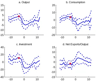
Figure 1 displays a typical default episode in our sample of emerging economies 12 quarters before and after defaulting (the Appendix describes the data and countries included). The values are reported as percentage deviations from trend calculated with the HP …lter (the standard smoothing parameter value of 1600 is used). Dotted lines correspond to plus- and minus-one-standard deviations around the mean. Relative to previous studies, the novel element in this …gure is the dynamics of investment.

One can see that investment follows a path that is qualitatively similar to the dynamics of output. For example, investment is above trend in the periods leading up to default, subsequently falling during default and remaining depressed for several quarters.6 _{On closer look, investment is}

far more responsive than output and consumption at the onset of the crises. Whereas consumption declines by 5 percent in the quarter of default, the collapse of investment is three times larger (15 percent). At the country level, the demise can be as large as -44 percent like in the 2001 Argentinean crisis. From peak to bottom, investment contracts by a whopping 27 percent (compare this with the milder decline in output of 8 percent). Clearly, investment does move substantially during default episodes. More important, this movement indicates that sovereign economies use investment to ameliorate the negative consequences of defaulting, i.e., to smooth out consumption.

5_{In the consumer …nance literature, several authors have examined the e¤ect of non-seizable wealth on default.}

Pavan (2008) studied an economy where households borrow and invest in durable goods. She explored several scenarios about what happens to the durable goods upon default. In her work, allowing lenders to seize a portion (rather than all) of the consumer’s durable goods increases the probability of default. Mitman (2011) found that bankruptcy rates are decreasing in the amount of home equity that can be retained after declaring bankruptcy. He further showed that, for a given level of net worth, more home equity increases the likelihood of declaring bankruptcy.

6_{Mendoza (2010) documents the decline of investment during sudden stops in several countries. His data set is}

-10 0 10 -15

-10 -5 0 5 10 15

a. Output

-10 0 10

-20 -10 0 10 20

b. Consumption

-10 0 10

-40 -20 0 20 40

c. Investment

-10 0 10

-15 -10 -5 0 5 10 15

d. Net Exports/Output

Figure 1: Average Default Episode in Emerging Economies.

A second interesting (and under-appreciated) feature of the data is that output and investment in emerging economies are typically growing above trend until four quarters before the default crisis. Moreover, these countries slowly return to trend, needing on average about 10 quarters to do so. Equally interesting, the transition to and from the default period is surprisingly smooth. Indeed, investment as well as output and consumption peak about four quarters (as indicated by the red circle) prior to reneging on debt. Further, the recovery is rather slow, taking an average of two years to return to trend.

3

Model

We modify CE’s long-term debt model to include labor and capital accumulation. Households consume, supply labor, and rank consumption/leisure bundles according to:

E0

1

X

t=0

t

u(ct; lt):

It is assumed a period utility of the type in Greenwood, Hercowitz, and Hu¤man (1988): u(ct; lt) =

(ct l

! t

!)

1 _{=(1 ). Production uses capitalk}

t and laborlt to produce outputytusing the

Cobb-Douglas function yt =Atktl

1

t . We assume that productivity follows logAt = (1 A) log A+ AlogAt 1+"A; where "A N(0; 2A).

Following CE, the sovereign government has access to long-term debt contracts, in which outstanding debt matures with probability . If debt does not mature, it delivers a coupon payment z. As shown by the authors, this debt structure not only captures the long-term nature of debt in the data but also helps improve the quantitative properties of the model without making its computation too onerous. Following the convention in the literature, we treat debt as negative wealth. Debt is chosen from a …nite set B R , which contains zero and strictly negative elements.7

A sovereign with debtbt<0may default. When it does so, four things happen. First, its debt

goes away. Second, he is excluded from credit markets upon default. Third, it is readmitted to credit markets with probability in the subsequent periods. Lastly, for the duration of autarky, a fraction of output is lost. This last assumption captures what is endogenized in MY, namely, that default impairs a country’s ability to produce by limiting its access to imports. Since capital refers to assets physically located within the borders of an economy, we further assume that capital cannot be expropriated in default and cannot be pledged as collateral.

Each period the sovereign decides whether to repay debt and, if so, how much new debt to issue subject to households’preferences, technology, and the economy’s resource constraint. The default decision is based on

V (bt; kt; mt; At) = max Vnd(bt; kt; mt; At); Vd(kt; At) ; (1)

where Vnd is the value of repaying debt (i.e., not defaulting) and Vd is the value of defaulting (and also the value of being excluded from credit markets). Consistent with our assumption of no expropriation, capital remains a state variable after default. A major di¤erence in our model relative to previous ones is that the default decision, and consequently the price of debt, depends on capital and productivity rather than an exogenous output level. In particular, the price of debt

7_{Default and debt maturity have been studied in recent superb contributions by Arellano and Ramanarayanan}

depends on the technology shock,At, the amount of debt,bt+1, and next period’s stock of capital,

kt+1: qt(bt+1; kt+1; At). Since qt is the price of debt to be repaid in the future, the relevant stock

of capital is the one that will be used to produce tomorrow, i.e., kt+1.8

The value of repaying debt is

Vnd(bt; kt; mt; At) = max ct;bt+1;it;kt+1;lt

u(ct; lt) + EtV (bt+1; kt+1; mt+1; At+1) (2)

subject to:

ct+qt(bt+1; kt+1; At)bt+1+it Atktl

1

t +mt

2 (kt+1 kt)

2

+ [ + (1 )z]bt+qt(bt+1; kt+1; At) (1 )bt;

it=kt+1 (1 )kt.

The right-hand-side term [ + (1 )z] captures payments from the fraction that matures and the coupon from the fraction(1 )that remains outstanding. The second termqt(bt+1; kt+1; At) (1 )

corresponds to the valuation of the outstanding debt at current bond prices. We incorporate the

iid term mt to facilitate the computation of the model. Following CE, this innovation is present

only in good standing and is drawn from a bounded normal with standard deviation m and

support [m; m]. The last equation is the law of motion of capital.

As already argued, a key contribution of this paper is the inclusion of capital accumulation in a way that captures the dynamics of investment found in the data. To this end, we found it necessary to include a variable adjusment cost (with parameter ) paid any time the capital stock deviates from its previous value. This is because, without adjustment costs, adverse productivity shocks result in two e¤ects that make investment ‡uctuate drastically. First, an adverse shock makes the sovereign want to smooth consumption by borrowing against higher expected productivity in the future. Second, such a shock also increases the sovereign’s default probability and so causes interest rates on debt to rise. Without adjustment costs, the cheapest way for the sovereign to “borrow” is by sharply reducing investment rather than borrowing on the world market. Consequently, investment ends up being too volatile relative to the series in the data. Adjustment costs make borrowing using capital more costly and so tame the ‡uctuations in investment.

It is worth noticing that the presence of an adjustment cost rather than its speci…c structure (ours follows Mendoza (1991)) is important to account for the dynamics of investment. In this sense, alternative formulations like those in Baxter and Crucini (1993), Christiano, Eichenbaum, and Evans (2005), and Nason and Rogers (2006) should work equally well. These speci…cations, however, make the cost a function of investment at time tand/ort 1, which greatly complicates

8_{Our price schedule shares some similarities with that in Bianchi, Hatchondo, and Martinez (2012). The authors}

the computation of an already involved model. The value of defaulting is

Vd(kt; At) = max ct;it;kt+1;lt

u(ct; lt) + (1 )EtVd(kt+1; At+1) + EtV (0; kt+1; mt+1; At+1); (3)

subject to:

ct+it (1 )Atktl

1

t

2 (kt+1 kt)

2

;

it = kt+1 (1 )kt.

As in the related literature, the sovereign is excluded from …nancial markets during the defaulting period t. With probability , the economy regains access to credit markets at t+ 1. In this case, the economy starts with zero debt. With probability 1 , it remains in autarky. Furthermore, upon default a fraction of production is lost. We assume that the loss of output during default depends on the state of the economy. In particular, the cost is

= max (0; d0+d1At):

Ours is a convenient modi…cation of the one considered in CE. The assumption that the cost depends on the state of technology (rather than output) greatly simpli…es the computation of our model.9 Since we are interested in the impact of capital on default and business cycles, we abstract from considerations about the structure of this cost and its implications for default models. We refer the reader to CE and MY for a vivid discussion on this very important issue.

For a debt level bt and capital stock kt, it is optimal to default for total factor productivity

(TFP) values and iid shock values in

D(bt; kt) = At; mt:Vnd(bt; kt; mt; At)< Vd(kt; At) : (4)

Similar to default models without capital, the sovereign reneges on his obligations only when

bt<0. The probability of default is then

pt(bt+1; kt+1; At) =

Z

D(bt+1;kt+1)

dF (At+1; mt+1jAt):

In the absence of capital, it is well understood that the default set shrinks withbt, i.e., lower debt

increases the likelihood of repayment (Arellano, 2008; CE; MY). The proof is straightforward be-cause debt a¤ects the default set (4) only through the good-standing value function (2). However,

9_{If we were to assume a function that depended on output ( = max (0; d}

0+d1yt)), solving for labor under

capital accumulation introduces several layers of di¢ culty to characterizeD(bt; kt). The …rst and

obvious obstacle is that the value functions Vnd and Vd may not be monotonic in capital due to the nonlinearity. Second, even with monotonicity for each value function, a change in the capital stock can have uneven e¤ects on the two value functions and cause the spread Vnd _Vd _{to vary}

nonlinearly. Hence, the inequality in (4) can easily reverse, complicating the characterization of the default set.

Foreign lenders are risk neutral. A zero pro…t condition implies that investors charge qt for

debt:

qt(bt+1; kt+1; At) =Et(1 dt+1(bt+1; kt+1; mt+1; At+1))

+ (1 ) [z+qt+1(bt+2; kt+2; At+1)]

1 +r ;

where dt+1 is an indicator function equal to 1 if the country defaults and 0 otherwise; r is the

risk-free international rate on a one-period bond.10

The presence of capital accumulation and long-term debt makes the computation of our model quite challenging. As a consequence, we follow Arellano (2008), CE and MY and abstract from the important issue of debt renegotiation. Bai and Zhang (2012) and Yue (2010) provide an excellent discussion of default and debt renegotiation.

3.1

Understanding Capital and Default

As argued in the previous paragraphs, capital accumulation introduces a nontrivial element to the default decision. To shed some light on the problem, let us consider the case where capital is an exogenous endowment, i.e., there is no investment decision. Further, suppose that the cost of default is constant, that the iid shockm is equal to zero, and that debt matures in one period,

= 1. Under these assumptions, the sovereign’s value of repaying its debt is

Vnd(bt; kt; At) = max ct;bt+1;ltf

u(ct; lt) + EtV (bt+1; kt+1; At+1)g

subject to

ct+qt(bt+1; kt; At)bt+1 Atktl

1

t +bt:

The value of defaulting is

Vd(kt; At) = max ct;lt

u(ct; lt) + (1 )EtVd(kt+1; At+1) + EtV (0; kt+1; At+1) ;

subject to

ct (1 )Atktlt1 :

10_{As in CE, we de…ne the "internal rate of return" as anr~(b}0_{; k}0_{; A)satisfyingq(b}0_{; k}0_{; A) = ( + (1 ) z)=( +} ~

r(b0_{; k}0_{; A)). The spreadrreported in the paper is then the annualized version ofr~minus the annualized risk-free}

One can easily show that, conditional on a level of capital, the model preserves the Eaton-Gersovitz property. That is, if the economy defaults for b, it will default for b0 < b 0, i.e.,

D(b; k) D(b0_{; k). This is because the value function of defaulting is independent of debt. A}

closer look at the value functions reveals that capital’s only role is to augment labor productivity.11

This observation highlights the complication behind characterizing the default set in the baseline model. Arellano (2008) provides an analytic description of the repayment decision in a model with iid endowment shocks. This assumption makes the analysis possible because expectations of tomorrow’s value functions are independent of today’s endowment (productivity) innovations. Allowing for persistent shocks, which has the same ‡avor as allowing for investment, breaks this independence, rendering an analytical exercise unfeasible. However, if we are willing to impose more structure, it is possible to sharpen the impact that capital has on default.

Proposition 1 Suppose that capital is an endowment that is either an iid shock or constant and

that productivity is iid. Further, let there be no output loss from default but assume the country is permanently excluded from international markets. If 0< <1 and ! > 1, then lower capital increases the temptation to default: for all k < ^k, if A₂D(b;k^) then A₂D(b; k).

Proof. See the Appendix.

We fall short of making a claim on the monotonicity of the default set with respect to capital in the general case when capital is a choice variable. We now turn to the calibration and the quantitative results to analyze the general case of endogenous capital accumulation.

4

Calibration

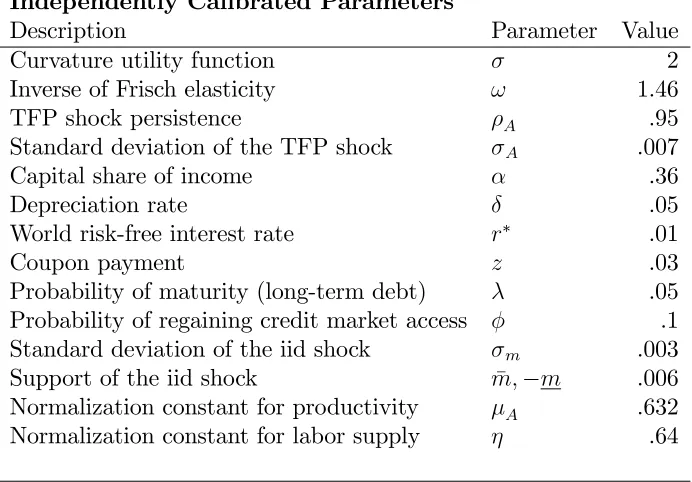
In our model, a period is a quarter. Our calibration approach follows closely the default literature. To this end, we divide the parameter space into two groups. The …rst group of parameters is set to values that have been previously used elsewhere (Table 1). Some of these parameters are worth mentioning. The structure of long-term debt is taken from CE with a coupon payment of

3 percent (z = :03) and a probability of maturity of 5 percent ( = :05) each quarter. CE base their selection on Argentinean data. The curvature of the utility function, , is set to a standard value of 2. The support of the continuous shock mt is the same as in CE. Following AG, the

probability of redemption is 10%, which corresponds to an average stay in autarky of 2.5 years. Conditional on the other parameters, we choose mean productivity _A and the labor disutility parameter so that, in the nonstochastic steady state without foreign lending, output and labor are both equal to one. The persistence and volatility of TFP are in line with the values used in the emerging-economy-business-cycle literature such as Fernandez-Villaverde et al. (2011), MY, and Neumeyer and Perri (2005).

11_{Indeed, the entire model can be recast, withA}

Independently Calibrated Parameters

Description Parameter Value

Curvature utility function 2

Inverse of Frisch elasticity ! 1.46

TFP shock persistence _A .95

Standard deviation of the TFP shock A .007

Capital share of income .36

Depreciation rate .05

World risk-free interest rate r .01

Coupon payment z .03

Probability of maturity (long-term debt) .05 Probability of regaining credit market access .1 Standard deviation of the iid shock m .003

Support of the iid shock m; m .006 Normalization constant for productivity _A .632 Normalization constant for labor supply .64

Table 1: Parameter Values Calibrated Independently

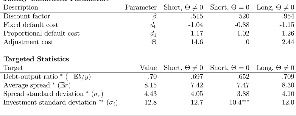
Table 2 reports the second set of parameters (discount factor, cost of adjusting debt, and cost of adjusting capital), which were chosen to match four empirical moments: debt-to-output ratio

( _Eb=y), average spread (_Er), volatility of spread ( r), and volatility of investment ( i). Except

for the standard deviation of investment, we exclusively target moments related to default. In this sense, our calibration exercise is very demanding. This is because we have one additional degree of freedom but the model’s …t includes three more moments related to the investment series. We further tie our hands by freezing the parameters of the TFP innovation to values used elsewhere. We defer the discussion of the calibration results to the next section. It su¢ ces for now to note that the parameters of the output loss function imply an asymmetric punishment of defaulting with a large loss if productivity is high, but low or zero loss if productivity is low. Our values are in line, although slightly larger (in absolute value) than those in CE.

5

Results

Jointly Calibrated Parameters

Description Parameter Short, ₆= 0 Short, = 0 Long, ₆= 0

Discount factor .515 .520 .954

Fixed default cost d0 -1.04 -0.88 -1.15

Proportional default cost d1 1.17 1.02 1.26

Adjustment cost 14.6 0 2.44

Targeted Statistics

Target Value Short, ₆= 0 Short, = 0 Long, ₆= 0

Debt-output ratio ( _Eb=y) .70 .697 .652 .709

Average spread (_Er) 8.15 7.42 7.47 8.30

Spread standard deviation ( r) 4.43 4.05 3.88 4.10

Investment standard deviation ( i) 12.8 12.7 10.4 12.0

Sample excludes 20 periods after default (following CE).

Full sample, series is logged and HP-…ltered before statistics are calculated. Volatility of ratio of investment to output (see main text for details).

Table 2: Parameter Values Calibrated Jointly

5.1

One-Period Debt Model

The column labeled "Short, ₆= 0" in Table 2 shows that the model with one-period debt is able to match the properties of the spread as well as the volatility of investment. This, however, comes at the price of an unrealistically low discount factor (0:515) and a large adjustment in capital accumulation to match the targeted statistics. The high impatience of the planner is a common feature of default models, but it is below the values reported in, for example, AG or MY. To understand this low value, recall that capital is a hedging instrument, so the planner can use it to smooth out consumption after adverse shocks. This means that, to induce defaults and hence match the volatility and mean of spreads in the data, the planner has to be very impatient.

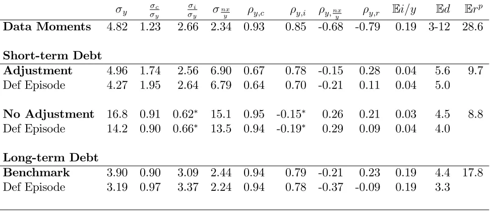
The upper panel of Table 3 presents the empirical moments from Argentina 1993.Q1 - 2011.Q3. A denotes a standard deviation, a denotes a correlation, and an _E denotes an average. Some of the empirical …ndings, such as the excess volatility of consumption ( c

y > 1) or the counter-cyclicality of the trade balance ( _y;nx

y ), have been extensively discussed elsewhere. Similarly, the probability of default (_Ed) has been reported to be in the range3percent to12percent on a yearly basis. Yet the excess volatility of investment ( i

y), its strong and positive correlation with output ( _yi), or the ratio of investment to GDP (_E(i=y)) are elements that have been overlooked in the default literature.

y _yc _yi nx_y y;c y;i y;nx_y y;r Ei=y Ed Erp

Data Moments 4.82 1.23 2.66 2.34 0.93 0.85 -0.68 -0.79 0.19 3-12 28.6

Short-term Debt

Adjustment 4.96 1.74 2.56 6.90 0.67 0.78 -0.15 0.28 0.04 5.6 9.7

Def Episode 4.27 1.95 2.64 6.79 0.64 0.70 -0.21 0.11 0.04 5.0

No Adjustment 16.8 0.91 0.62 15.1 0.95 -0.15 0.26 0.21 0.03 4.5 8.8

Def Episode 14.2 0.90 0.66 13.5 0.94 -0.19 0.29 0.09 0.04 4.0

Long-term Debt

Benchmark 3.90 0.90 3.09 2.44 0.94 0.79 -0.21 0.23 0.19 4.4 17.8

Def Episode 3.19 0.97 3.37 2.24 0.94 0.78 -0.37 -0.09 0.19 3.3

Since investment series is sometimes negative,i=y is used in place of logi.

Note: the entire sample is used. Data for and are logged and HP-…ltered except for r. and nx=y. _Erp _{is the average interest rate just prior to default.}

Table 3: Moments in Data and Model

model captures the qualitative properties found in the Argentinean sample. The model, however, generates some anomalies. For example, since changing capital is costly, capital cannot be fully adjusted to smooth out consumption over the business cycle. As a consequence, consumption displays too much volatility relative to the data. This excessive volatility in turn translates into 1) a low correlation between output and consumption, y;c = 0:67, and 2) counterfactually large

‡uctuations in the trade account, nx

y = 6:9. A second drawback of the model is its prediction of too low average capital accumulation as re‡ected by the low investment-to-output ratio (4percent in the model versus 19 percent in the data). We defer the discussion of the positive correlation between output and interest rates until the next section. It su¢ ces for now to note that this re‡ects the sovereign’s incentives to borrow when productivity is high.

The third row (Def Episode) in Table 3 shows the model’s moments prior to a default crisis. To this end, we do a long simulation of the model, locate the default events, and then compute the moments using the 74 observations leading up to (but excluding) the default period (this is the same approach in, Arellano, 2008). The table reports the average across all, the events. Conditioning on this episode does not change the predictions of our model.

correlation of this ratio with GDP in lieu of the ratio of volatilities and the correlation between output and investment.

The solid lines in Figure 2.a display the dynamics around default in the one-period debt model when capital accumulation is costly. For clarity, we also plot one-standard-deviation bands (dashed lines). Contrary to the data, the model predicts a boom-bust cycle, which is characteristic of default models. That is, the small open economy peaked just before reneging on its international obligations. Indeed, default in the model results from a large negative productivity shock, which was preceded by a positive innovation.

-15 -10 -5 0 5 10 15

-20 0 20

a. Output

-15 -10 -5 0 5 10 15

-20 0 20

b. Consumption

-15 -10 -5 0 5 10 15

-20 -10 0 10

e. Labor

-15 -10 -5 0 5 10 15

-20 -10 0 10

d. Net Exports/Output

-15 -10 -5 0 5 10 15

-40 -20 0 20 40

c. Investment

-15 -10 -5 0 5 10 15

-3 -2 -1 0 1 2

f. Productivity

Figure 2.a: Default Episode in the One-Period Debt Model with Adjustment Cost

-15 -10 -5 0 5 10 15 -50

0 50

a. Output

-15 -10 -5 0 5 10 15

-50 0 50

b. Consumption

-15 -10 -5 0 5 10 15

-50 0 50

e. Labor

-15 -10 -5 0 5 10 15

-20 0 20

d. Net Exports/Output

-15 -10 -5 0 5 10 15

-40 -20 0 20 40

c. Investment/Output

-15 -10 -5 0 5 10 15

-2 0 2

f. Productivity

Figure 2.b: Default Episode in One-Period Model without Adjustment Cost

To Summarize, the model with short-term debt seems to capture some of the relevant features of the data. However, this only possible if one accepts that emerging economies are extremely impatient. Leaving aside the degree of patience, our simulations also point to adjustment costs of capital being an essential ingredient of the model. With these …ndings in place, we now show that long-term debt goes a long way toward bringing the model closer to the data while using more conventional parameter values.

5.2

Long-Term Debt Model

The column "Long, ₆= 0" in Table 2 shows that our baseline model matches the targeted moments with a more realistic discount factor and a lower adjustment cost in capital. At …rst sight, this …nding is surprising because the central planner is more patient and can move capital more freely in response to shocks. These two factors by themselves should reduce the temptation to default and hence decrease the mean and volatility of spreads. However, the planner tends to over-accumulate long-term debt because it can be easily rolled over. Since the cost of borrowing is increasing in the stock of debt, this excessive long-term borrowing increases the temptation to default even though the planner is fairly patient.12

Overall, our calibrated model does a better job matching Argentina’s business cycles (last panel in Table 3). We capture simultaneously the large ‡uctuations of output and the volatility of

net exports. Although the model correctly predicts the countercyclicality of the trade account, we fall short of delivering its magnitude (this is also the case in the work of Arellano, 2008; CE; and Mendoza and Yue, 2011). Crucially, these results come from a model that uses a more plausible discount factor. The default probability is 4.4 in our model, which is similar to what we …nd with the one-period debt model. The value falls within the range of the frequency of default in Argentina reported in the literature.

More relevant to our purpose, the model gets close to replicating the correlation of investment and output. Consistent with the data, the model predicts a ratio of investment to output of

19 percent. Matching the average investment in the data is crucial because, in the spirit of incomplete market models (Aiyagari, 1994), the sovereign country can use capital to hedge against bad outcomes. That is, having more capital ameliorates the cost of defaulting because capital can be freely transformed into consumption goods. Our benchmark model predicts an average capital-to-output ratio of 3:83 (this is the mean of the ergodic distribution).13 _{In contrast, this ratio is}

3:66 in the steady state of our model that excludes default and foreign borrowing (4:5 percent lower).

There are two dimensions in which the model does not quite match the data. Similar to the one-period debt model, our fully blown model predicts a positive correlation between output and interest rates. This …nding indicates the strong RBC ‡avor of the model. To see this, recall that in the RBC model the return on capital is positively correlated with output. In our model, the return of capital and sovereign debt are closely connected because they have very similar return structures resulting in close-to-arbitrage opportunities. As a consequence, the resulting correlation lives somewhere between the pure default and pure RBC realms.

A second counterfactual feature of the model is that the volalitity of consumption is lower than that of output. A lesson from the one-period debt model is that having access to capital is not enough to deliver the prediction of smooth consumption. This is because the planner can fully counteract adverse productivity shocks when the savings tool, i.e., capital, is completely ‡exible. Issuing long-term debt restores this ‡exibility in the presence of costly capital. We show later on that the model does predict excess volatility in consumption if one is willing to reduce the elasticity of labor supply in the model.

We now turn to the implications of capital accumulation on the price of debt. Figure 3 shows the bond price schedule along the capital and bond dimensions conditional on a typical productivity shock. For a given capital value, we obtain the standard result that lower levels of debt are associated with higher bond prices (in our …gures, debt is expressed as a fraction of output in steady state, which we normalize to 1). More importantly, the …gure reveals one crucial

13_{Even taking into account a debt-output ratio of .71, this number still seems high as it results in a wealth-output}

result of this paper: Additional capital helps sustain higher levels of debt.

Figure 3: Bond Price with Typical Productivity

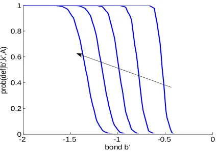
To further underscore the last point, Figure 4 plots the price schedule for …ve di¤erent levels of capital: the lowest capital stock in our grid, the 25th percentile, the 50th percentile, the 75th percentile, and the largest stock of capital (the arrow indicates the direction in which capital increases). At the lowest capital level, debt (as a fraction of steady-state output) starts having some value at aroundb = 0:70. At the other extreme, when capital is at its highest level (farthest northwest line), debt has a positive price at a debt value of around b = 1:6. This is more than twice (in absolute terms) as large as its value when capital is low. Figure 4 also indicates that the stock of capital today raises the price of debt for any debt level. Even when the sovereign issues a very small amount of debt, the price of debt still increases with capital holdings. The e¤ect is more pronounced for higher values of debt. This observation may help explain in part why more developed— that is, more heavily capitalized— countries are able to support higher debt-output ratios than less developed countries.

increments (50th to 75th percentile and 75th to 100th percentile), the impact on price diminishes to a mere 3 percent (1.127 to 1.164) and 2 percent (1.164 to 1.187) , respectively.

The evolution of the price schedule as capital varies highlights the two tensions that capital in‡icts on the decision to default. At low levels of capital, each additional unit gives the planner more ‡exibility to smooth out adverse shocks. The country is then more likely to repay its obliga-tions and hence lenders are willing to lend at low spreads. However, as the economy accumulates more capital, default becomes more attractive since the value of autarky is increasing on the stock of capital at default. Lenders internalize these two forces by increasing the price of debt when capital increases but increasing it less if capital is already high. A crucial insight from this analysis is that, by varying the stock of capital, emerging economies could, in principle, select the region of the price schedule at which they want to borrow.

-2

-1.5

-1

-0.5

0

0

0.2

0.4

0.6

0.8

1

1.2

1.4

bond b'

p

rice

q

(b

',k',A)

Figure 4: Bond Price at Di¤erent Capital Levels

Figure 5 compares the price schedules for the lowest productivity (blue solid lines) and the highest productivity in our grid (red dashed lines). We plot the price schedules for three levels of capital for each productivity level (capital increases as we move in the northwest direction). From this …gure, we observe that higher productivity ampli…es uniformly the e¤ect of capital holdings on debt sustainability and bond pricing: Capital always increases the price of debt, but the price increase is larger when productivity is high.

smoothing channel) on debt prices. The …rst is that capital increases resources to repay much more when productivity is high than when productivity is low. The second is that productivity is persistent, implying that low productivity today results, typically, in low productivity tomorrow. With low TFP persisting into the future, increased capital has only a marginal e¤ect on future income and ability to repay. This second e¤ect is absent in the one-period debt model.

-30 -2.5 -2 -1.5 -1 -0.5 0 0.2

0.4 0.6 0.8 1 1.2 1.4

bond b'

p

ri

ce

q

(b

',

k',A

)

Lowest A Highest A

Figure 5: Bond Price with Highest and Lowest Productivity

-2

-1.5

-1

-0.5

0

0

0.2

0.4

0.6

0.8

1

bond b'

prob(d

ef|

b',k

',A

)

Figure 6: Probability of Default at Di¤erent Capital Levels

-10 0 10 -30

-20 -10 0 10

a. Output

-10 0 10 -20

-10 0 10

b. Consumption

-10 0 10 -20

-10 0 10

e. Labor

-10 0 10 -10

0 10

d. Net Exports/Output

-10 0 10 -60

-40 -20 0 20

c. Investment

-10 0 10 -5

0 5

f. Productivity

Figure 7: Default Episode in Model

Interestingly, our model predicts that, on average, the economy is in trade balance (i.e., net exports are zero) when default is declared and then experiences a mild trade de…cit. To understand this subsequent worsening of the trade account, …rst note that net exports in the economy can be written as N Xt =qt(bt+1; kt+1; At)(bt+1 (1 )bt) ( + (1 )z)bt. When a sovereign defaults

at time t, bt is set to 0 and, for as long as the sovereign remains in autarky, both bt+1 and N Xt

are 0. When the economy is readmitted to …nancial markets, say, at time , b +1 is chosen from

B R and so N X must be less than 0.14

The model also predicts an improvement of the trade balance prior to declaring default. This is explained by …rst noting that higher productivity and capital (due to additional investment) occur during the pre-crisis periods. Second, note that, as shown in Figures 4 through 6, the bond price schedule is increasing both in productivity and capital. Indeed, new debt is barely discounted for small enough levels of existing debt. Consequently, in the pre-crisis periods the sovereign can meet its …nancial obligations with only a small issuance of debt, resulting in a trade surplus. At …rst sight, this prediction seems at odds with the average default episode in the data. However, it

14_{This is a feature common to most sovereign default models. An exception is that of Mendoza and Yue (2011),}

is consistent with the default episodes of Indonesia (1998.Q3), Peru (1983.Q2), and South Africa (1998.Q1). Furthermore, Arellano (2008) and Mendoza and Yue (2011) report similar dynamics prior to default.

5.3

Dissecting the Role of Capital

As discussed above, capital brings two tensions to the model. More capital gives the planner a savings tool to weather bad times and either avoid or postpone default. But it also increases the bene…t of defaulting since the value of autarky rises with capital. To illustrate these forces, we plot in Figure 8 the value functions of repayment (Vnd_{; left panel), default (V}d_{; right upper panel),}

and their di¤erence (Vnd _Vd_{; right bottom panel) as a function of capital for three levels of debt.}

All …gures are conditional on median productivity and the median m shock.

The interplay between debt and capital is nontrivial. For instance, when a country is deeply indebted (solid blue line in Figure 8), additional capital improves the sovereign’s ability to repay faster than it improves the value of autarky. This is re‡ected in the spread Vnd Vd being universally increasing in k. This spread, however, is concave ink.

To have some intuition about these results, consider what the envelope conditions ofVnd _and

Vd _{would be if leisure were not valued, there was one-period debt, and the problem was smooth:}

V_knd =u0(cnd)(1 +A k 1 ) and V_kd=u0(cd)(1 + (1 )A k 1 ):

For su¢ ciently large debt levels, cnd cd and so V_knd V_kd > 0. Consequently, the spread is increasing in capital. The reason the spread is concave is that, ask increases,cnd _{tends to respond}

faster than cd _{for two reasons. First, conditional on repaying, marginal utility today is quite}

high, so the sovereign would like to lower it by “eating” much of the capital. Second, conditional on repaying, the sovereign gets to keep all additional output, whereas conditional on default, fraction is lost. Hence u0_(cnd_{) decreases faster than u}0_(cd_{). Moreover, (1 +A k} 1 _{) decreases}

faster than (1 + (1 )A k 1 _{). Consequently, V}nd

k decreases faster in k than Vkd decreases,

and so the spread is concave.

The story is somewhat di¤erent at low levels of debt (dotted black line). There, the sovereign already has a near perfect ability to repay the small amount of debt. Consequently,cndtends to be much higher thancd_{and so the marginal bene…t of capital is higher for the sovereign that defaults}

(Vnd

k Vkd<0). In other words, the smoothing channel of increased capital is nearly absent (Vknd is

small) and the autarky channel dominates (Vd

k is large). Hence the spread isdecreasing in capital.

The convexity of the spread is an empirical …nding that is more di¢ cult to explain.15

In a one-period debt framework, how the spread Vnd _Vd _{responds when debt is low would}

suggest that, if anything, the price of small levels of debt should decrease as capital increases. Why, then, does the opposite result obtain? It is because debt is long term. High capital today results in higher average levels of capital several periods in the future when, typically, the country will be more indebted. It is there where additional capital, resulting in reduced future default probabilities, comes to bear and results in a higher price today.

2 4 6 8

-100 -90 -80 -70 -60 -50 -40

k

Vnd

Vnd, B = -1.5 Vnd, B = -0.5 Vnd, B = 0

2 4 6 8

-100 -80 -60 -40

Vd

k

2 4 6 8

-5 0 5 10 15

Vn

d - V

d

k

Figure 8: Value Functions of Repayment (Vnd) and Default (Vd)

An alternative way to isolate these e¤ects is by studying an economy in which investment follows a policy rule outside the planner’s control. Under this assumption, investment loses its smoothing feature and retains only its role in increasing resources available upon default. Ana-lyzing this scenario requires two steps. First, we obtain an exogenous investment policy function

15_{Since the sovereign that repays gets to keep all its output,c}nd_{potentially responds faster to an increase ink}

by solving an RBC version of our model where the sovereign chooses any k0 but cannot borrow, i.e., b0 = 0. For technical reasons, we assumed that this k0 applied to the entire interval [m; m], and that the sovereign chose it assuming m = m.16 _{In the second step, we use this exogenous}

investment policy function, together with the autarky value and autarky capital policy from the benchmark, but allow the sovereign to optimally choose b0 _{and for prices to respond. Once again,}

we assumed that the b0 _{applied to the entire interval and that it was chosen assuming m=m.}17

-15 -10 -5 0 5 10 15

-30 -25 -20 -15 -10 -5 0 5 10

Benchmark Exogenous Capital

Figure 9: Investment Dynamics Around Default

Figure 9 displays the dynamics of investment during default for both the benchmark model (solid line) and when capital is exogenously determined (dashed line). As expected, the planner in the benchmark model exploits investment in the periods prior to default. Note that, in an attempt to ameliorate the impact of adverse shocks on consumption, investment (and hence capital) has been declining for a few quarters by the time the country moves to autarky. In contrast, when investment is not a choice variable, the central planner defaults when the stock of capital is at its highest level. This is because the planner only internalizes the bene…t that capital has on the value of autarky. It is better to run away when capital is high because it gives the economy a boost when excluded from international markets. What the planner would like to do is liquidate

16_{When the sovereign is forced to use an exogenous capital policy that varies across the m interval, then the}

value function is no longer guaranteed to be increasing in m, which our computational algorithm assumes.

17_{These assumptions resulted in the value function iteration not converging. Since these cases are just for}

y _yc _yi nx_y y;c y;i y;nx_y y;r Ei=y Ed Erp

Data Moments 4.82 1.23 2.66 2.34 0.93 0.85 -0.68 -0.79 0.19 3-12 28.6

Long-term Debt

Exogenous k 3.51 1.17 2.03 1.69 0.88 0.84 -0.28 0.17 0.18 4.5 21.6

Def Episode 2.83 1.29 2.10 1.55 0.91 0.72 -0.47 -0.15 0.18 3.2

Low Elasticity 2.17 1.20 4.03 2.58 0.74 0.76 -0.25 0.23 0.19 4.3 16.8

Def Episode 1.79 1.35 4.42 2.37 0.77 0.73 -0.39 -0.09 0.19 3.3

Benchmark 3.90 0.90 3.09 2.44 0.94 0.79 -0.21 0.23 0.19 4.4 17.9

Def Episode 3.19 0.97 3.37 2.24 0.94 0.78 -0.37 -0.09 0.19 3.3

Note: Entire sample used, except when stated o/w. All and are with logged and HP-…ltered data except r and nx=y.

Table 4: Moments in Data and Model

some capital in order to smooth consumption and avoid default, but he cannot as investment is outside his control.

The crucial smoothing role of investment prior to default is further exposed in Table 4. There we compare the dynamic properties of the model with exogenous capital accumulation and those of the benchmark scenario. Despite investment being volatile as in the benchmark model, the planner’s inability to adjust investment results in a lower investment-to-GDP ratio and less consumption smoothing: Consumption volatility is considerably higher. This excess volatility in turn reduces the correlation between output and consumption.

5.4

Volatility of Consumption

Our benchmark model predicts counterfactually smooth consumption dynamics. An obvious ques-tion, then, is whether this is a general feature of our model or an artifact of the very demanding calibration strategy (recall that our model is calibrated using only four parameters but we tested it along many dimensions). We …nd that the latter explanation is more plausible for three reasons. First, the one-period debt version does generate excess consumption volatility, so if we were to shorten the duration of the long-term debt contract, then the excess volatility could be obtained. Second, if we reduce the labor supply elasticity, and thereby reduce the planner’s ability to re-spond to shocks, we …nd the volatility of consumption moves in the right direction ( c= y = 1:20)

ver-sion of this paper (Gordon and Guerron-Quintana, 2012), we show that if we target a few more moments like the volatility of consumption and output, the resulting model does a better job matching business cycle statistics and default episodes. However, in this paper we have chosen a very stringent calibration procedure to make our model as comparable as possible to previous work, thus highlighting the role of capital.

6

Conclusion

In this paper, we propose a model with endogenous sovereign default and capital accumulation. The model is parsimonious, but captures key moments in the data. We …nd that more capital reduces the likelihood of default and hence increases the price of sovereign debt. Interestingly, the impact of capital on either the price of debt or the probability of default displays diminishing returns.

Our simulations indicate that both long-term debt and adjustment costs to capital are crucial ingredients to match simultaneously default and business cycle properties. The assumption of long-term debt is quite natural, as countries can and do issue long-long-term obligations. The assumption of costly capital adjustment in our model is also shared by most international business cycle models and is needed to match the dynamics of investment. This is because the cost prevents the sovereign from freely adjusting capital. Since investment decisions are typically made by households, we view this adjustment cost as a reduced-form way of capturing the planner’s di¢ culty in inducing households to choose investment properly. What would happen if the sovereign had to instead solve a Ramsey problem to induce optimal investment is an interesting question that should be investigated in future research.

References

[1] Aguiar M., and G. Gopinath (2006). "Defaultable Debt, Interest Rates and the Current Account," Journal of International Economics 69, 64-83.

[2] Aiyagari R. (1994). "Uninsured Idiosyncratic Risk and Aggregate Saving," Quarterly Journal of Economics 109, 659-684.

[3] Arellano C. (2008). Default Risk and Income Fluctuations in Emerging Markets. American Economic Review 98, 690-712.

[4] Arellano C., and Y. Bai (2012). Linkages Across Sovereign Debt Markets. Mimeo, University of Rochester.

[6] Bai Y., and J. Zhang (2012). Duration of Sovereign Debt Renegotiation. Journal of Interna-tional Economics 86, 252-268.

[7] Baxter M., and M. Crucini (1993). Explaining Saving-Investment Correlations. American Economic Review 83, 416-436.

[8] Bianchi J., J.C. Hatchondo, and L. Martinez (2012). International Reserves and Rollover Risk. Mimeo University of Wisconsin.

[9] Chatterjee S., and B. Eyigungor (2011). Maturity, Indebtedness, and Default Risk. Federal Reserve Bank of Philadelphia, Working paper 11-33.

[10] Crego A., D. Larson, R. Buter, and Y. Mundlak (1998). A New Database on Investment and Capital for Agriculture and Manufacturing. World Bank.

[11] Christiano L., M. Eichenbaum, and C. Evans (2005). Nominal Rigidities and the Dynamic E¤ects of a Shock to Monetary Policy." Journal of Political Economy 113, 1-45.

[12] Fernandez-Villaverde J., P. Guerron-Quintana, J. Rubio-Ramirez, and M. Uribe (2011). Risk Matters: The Real E¤ects of Volatility Shocks. American Economic Review 101, 2530-2561.

[13] Gordon G. and P. Guerron-Quintana (2012). Dynamics of Investment, Debt, and Default. Mimeo Department of Economics, Indiana University.

[14] Greenwood J., Z. Hercowitz, and G. W. Hu¤man (1988). Investment, Capacity Utilization, and the Real Business Cycle. American Economic Review 78, 402-417.

[15] Hatchondo J.C., and L. Martinez (2009). Long-Duration Bonds and Sovereign Defaults. Jour-nal of InternatioJour-nal Economics 79, 117-125.

[16] Hatchondo J.C., L. Martinez, and H. Sapriza (2010). Quantitative Properties of Sovereign Default Models: Solution Methods Matter. Review of Economic Dynamics 13, 919-933.

[17] Kamps C. (2004). New Estimates of Government Net Capital Stocks for 22 OECD Countries 1960-2001. IMF Working Paper 04/27.

[18] Kehoe P. and F. Perri (2002). International Business Cycles with Endogenous Incomplete Markets. Econometrica 70, 907-928.

[19] (2004). Competitive Equilibria with Limited Enforcement. Jour-nal of Economic Theory 119, 184-206.

[21] (2010). Sudden Stops, Financial Crises, and Leverage. American Economic Review 100, 1941-1966.

[22] , and V. Yue (2011). A General Equilibrium Model of Sovereign Default and Business Cycles. NBER, Working paper 17151.

[23] Mitman K. (2011). Housing and the Macroeconomy: The Role of Bailout Guarantees for Government Sponsored Enterprises. Mimeo University of Pennsylvania.

[24] Nason J., and J. Rogers (2006). The Present-value Model of the Current Account has been Rejected: Round up the Usual Suspects. Journal of International Economics 68, 159-187.

[25] Neumeyer A., and F. Perri (2005). Business Cycles in Emerging Economies: The Role of Interest Rates. Journal of Monetary Economics 52, 345-380.

[26] Park J. (2012). Sovereign Default Risk and Business Cycles of Emerging Economies: Boom-Bust Cycles. Unpublished Manuscript, University of Wisconsin Economics Department.

[27] Roldan J. (2012). Default Risk and Economic Activity: A Small Open Economy Model with Sovereign Debt and Default. Unpublished Manuscript, Banco Central de Mexico.

[28] Pavan M. (2008). Consumer Durables and Risy Borrowing: The E¤ects of Bankrupcy Pro-tection. Journal of Monetary Economics 55, 1441-1456.

[29] Reinhart C., and K. Rogo¤ (2008). This Time is Di¤erent: A Panoramic View of Eight Centuries of Financial Crises. NBER Working Paper 13882.

[30] Uribe M., and V. Yue (2006). Country Spreads and Emerging Countries: Who Drives Whom? Journal of International Economics 69, 6-36.

[31] Yue V. (2010). Sovereign Default and Debt Renegotiation. Journal of International Economics 127, 889-946.

7

Appendix

7.1

Data Description

For the business cycle statistics, data are collected from the International Financial Statistics and OECD’s statistical database. Figure 1 is generated using the following countries: Argentina (1993.Q1-2011.Q3; 2002Q1), Ecuador (1991.Q1-2002.Q2; 1999Q3), Indonesia (1997.Q1-2011.Q3; 1998.Q3), Mexico (1981.Q1-2011.Q3; 1982.Q4), Peru (1979.Q1-2011.Q3; 1983.Q2), Philippines (1981.Q1-2011.Q2; 1983.Q4), Russia (1995.Q1-2011.Q3; 1998.Q4), South Africa (1960.Q1-2011.Q3; 1985.Q4 and 1993.Q1), and Thailand (1993.Q1-2011.Q2; 1998.Q1). The …rst numbers for each country correspond to the sample length while the second observation indicates the year and quarter of default.

The variables were seasonally adjusted. Nominal variables were de‡ated by the GDP de‡ator. All variables except net exports were expressed in logs. Finally, the HP …lter with smoothing parameter 1600 was used to detrend all observations.

7.2

Proofs

Lemma 1. Suppose that capital is an endowment that is either an iid shock or constant and that

productivity is iid. Further, let there be no output loss from default but assume the country is permanently excluded from international markets. Then, the problem can be recast as the model of Arellano (2008), where the endowment is y~, a function of only A and k:

~

y=F(A; k):

Moreover, y~is iid.

Proof. The sovereign’s value of not defaulting is

Vnd(bt; kt; At) = max ct;lt;bt+1

u ct

~

lt !

! !

+ _EV(bt+1; kt+1; At+1)

subject to ct+qt(bt+1)bt+1 =Atktl

1

t +bt

and of defaulting is

Vd(kt; At) = max ct;lt

u ct

~

lt !

! !

+ _EVd(kt+1; At+1)

subject toct=Atktl

1

t

where

V(bt+1; kt+1; At+1) = max Vnd(bt+1; kt+1; At+1); Vd(kt+1; At+1) :

The optimal choice is

e lt=

1

Atkt

1 +! 1

: (5)

De…ne an auxiliary variable ~ct = ct

~

l!t

!. This is consumption net of labor disutility. Further,

de…ne

e

yt =Atkt~l

1 t ~ lt ! ! :

The sovereign’s problems can now be rewritten as

Vnd(bt;y~t) = max

~

ct;bt+1

u(~ct) + EV(bt+1;y~t+1)

subject to ~ct+qt(bt+1)bt+1 = ~yt+bt

and

Vd(~yt) = max

~

ct

u(~ct) + EVd(~yt+1)

subject to~ct= ~yt

where

V(bt+1;y~t+1) = max Vnd(bt+1;y~t+1); Vd(~yt+1) :

Since y~inherits the iid properties ofA andk, this is the same setup as in Arellano (2008) (with ~c

as consumption and y~as the endowment).

Proposition 1. Suppose the conditions of Lemma 1 are met. If 0< <1 and ! >1, then

lower capital increases the temptation to default: for all k <k^, if A ₂D(b;^k) then A₂D(b; k).

Proof. Since Arellano (2008) proves the default set is decreasing in y~t (Proposition 3), we can

apply Lemma 1 to show the default set is decreasing in kt if y~t is increasing in kt. It su¢ ces to

show that y~t is increasing inAtkt:

@y~t

@Atkt

= ~l1_t +Atkt(1 )~lt

@~lt

@Atkt

~_l! 1

t

@~lt

@Atkt

= ~l1_t + @ ~_lt

@Atkt

Atkt(1 )~lt ~l ! 1

t

= ~l1_t + @ ~_lt

@Atkt

~

l_t Atkt(1 ) ~l

+! 1

t

= ~l1_t + @ ~_l

t

@Atkt

~

l_t Atkt(1 )

1

Atkt * Eqn. (5)

= ~l1_t

7.3

Computational Algorithm

As emphasized in CE, long-term debt models su¤er from convergence problems that can be miti-gated by including a continuous iid shock in the computation. In fact, the convergence problems are even worse when capital is introduced. Relying on monotonicity of the policy function, CE construct a computational algorithm to explicitly handle a continuous shock. Unfortunately, with two assets, bonds and capital, we do not have a proof of monotonicity. However, we now present a computational algorithm that does not rely on monotonicity and can be trivially extended to a general choice set. As the only non-trivial part of the computation is incorporating a continuous iid shock, we focus on this part of the computation.18

For compactness, we switch to recursive notation with a “0 _{”denoting next period’s value and}

useainstead of A. The algorithm’s objective is, for a given(b; k; a), to …nd policiescnd_{(b; k; m; a),}

b0nd_{(b; k; m; a), k}0nd_{(b; k; m; a), and V}nd_{(b; k; m; a) for all m}

2 [m; m] such that the budget set is nonempty. To this end, we …x (b; k; a), suppress dependence on it, and begin with the following de…nitions:

1. De…neX =_f(b0_{; k}0_)j(b0_{; k}0_{)2B Kgwith typical elementx= (b}0_{; k}0_{). X is the choice space.}

2. De…ne c:X _!R by

c(x) = q(b0; k0; a)(b0 (1 )b) + ( +z(1 ))b k0+ (1 )k

2(k

0 _k)2

+ak l(k; a)1 l(k; a)

!

! :

c(x) is the consumption— net of labor disutility and m— arising from a choice of x. Note that we have writtenl(k; a)using the convenient Greenwood, Hercowitz, and Hu¤man (1988) property.

3. De…ne W :X_!R by

W(x) = _EV(b0; k0; m0; a0):

W is the continuation utility associated with the choice of x.

4. De…ne X~(m) X by

~

X(m) =_fx₂X_jc(x) +m 0_g:

~

X(m) contains all feasible choices of X given m. Note that X~(m1) X~(m2) whenever

m1 < m2.

5. De…ne V(x; m) for all m and x₂X~(m) by

V(x; m) = u(c(x) +m) +W(x):

18_{Hatchondo, Martinez and Sapriza (2010) discuss alternative methods and their accuracy to solve models of}

Then V represents the indirect utility from choicex given the current state and some shock

m.

By de…nition, we have

xnd(b; k; m; a)₂arg max

x2X~(m)

V(x; m)

cnd(b; k; m; a) = c(xnd(b; k; m; a)) +m+ l(k; a)

!

! ; and Vnd(b; k; m; a) =V(xnd(b; k; m; a); m);

which are well de…ned if and only if X~(m) is nonempty.

We now simplify the discussion of the algorithm by providing some theoretical results:

Lemma 2 V(x1; m) = V(x2; m) for all feasible m if and only if c(x1) = c(x2) and W(x1) =

W(x2).

Proof. Since V is di¤erentiable inm, we have

V(x1; m) =V(x2; m),

9m s:t: V^ (x1;m^) = V(x2;m^) and

@V(x1; m)

@m =

@V(x2; m)

@m 8m:

Because @V(x; m)=@m = u0(c(x) +m), the second part is true if and only if c(x1) =c(x2). The

…rst part is true for c(x1) =c(x2)if and only if W(x1) =W(x2).

Lemma 3 Given two choices x1 and x2, fmjV(x1; m) = V(x2; m) and x1; x2 2 X~(m)g is either

empty, a singleton, or equal to [ c(xi);1) for bothi= 1 and2. If c(x1)6=c(x2), then it is either empty or a singleton and so V(x1; ) and V(x2; ) cross at most once.

Proof. For all m such that x1; x2 2 X~(m), de…ne H(m) =V(x2; m) V(x1; m). Then H0(m) =

u0_(c(x

2) +m) u0(c(x1) +m). It is then obvious thatH0(m)never changes sign, and soH(m)has

at most one zero (or is always zero if c(x1) =c(x2)by Lemma 2).

Proposition 4 Let (x ; m ) be such that m ₂[m; m], V(x ; m ) V(x; m ) for all x₂X~(m ),

and, if V(x ; m ) =V(x; m ), thenc(x ) c(x). Then x is optimal for allm in [m ; m ] where

m :=

(

max_f c(x ); m_g if _fx_jc(x)> c(x )_g is empty

max c(x ); m;max_fxjc(x)>c(x )gm~(x) otherwise

and m~(x) is de…ned implicitly by

Further, m~(x) is well de…ned (unique and exists) for each x having c(x) > c(x ) and lies in the interval ( c(x ); m ).

Proof. De…nem^ := max_f c(x ); m_g. Then x is feasible for all m m^.

First we prove that, for m ₂[ ^m; m ], any x₂ X~(m ) with c(x) c(x ) delivers weakly lower utility than x or is not feasible. Note that, where feasible, @V(x; m)=@m @V(x ; m)=@m. Consequently, for m m wherex is feasible, we haveV(x; m) V(x ; m). Moreover, wherex is feasible, x is feasible.

Now consider an x with c(x) > c(x ). Then where x is feasible, x is feasible. So we have

@V(x; m)=@m < @V(x ; m)=@m for all m ₂ ( ^m; m ]. Further, there exists an m~ ₂ ( c(x ); m )

s.t. V(x;m~) = V(x ; m) because, as m _# c(x ), V(x ; m) _{# 1} for the preferences we have chosen while V(x; m)is not arbitrarily negative. Then by virtue of the single crossing property of

V(x; m) V(x ; m)(see Lemma 3), we have V(x ; m) V(x; m) for all m₂[max_fm;~ m^_g; m ]. Let the m~ for x with c(x) > c(x ) be denoted m~(x). De…ne, when there is at least one x s.t.

c(x)> c(x ), m = max_fm;^ max_fxjc(x)>c(x )gm~(x)g. Otherwise, de…ne m = ^m. Then from the

preceding arguments we have V(x ; m) V(x; m)₈m₂[m ; m ].

The preceding proposition suggests a natural algorithm for computing the optimal policy. Beginning with the optimal choice at m, iterate down until one has reached m (or exhausted feasible choices). We state it formally now:

Algorithm

Objective

Compute the optimal policy and value function. Initialization

If X~(m) = _;, then no feasible policies exist for any m ₂ [m; m] and we are done, so STOP. Otherwise, de…ne m₁ =m. Set i= 1 and go to Step 1.

Step 1

For all x ₂ X~(m₁), compute V(x; m₁): Let x_{1 2} argmaxV(x; m₁) such that if the arg max is not a singleton, then x₁ has the smallest value of c(x). If even this is not unique, employ a tie-breaking rule as Lemma 2 implies the choices o¤er the same utility everywhere.

One may proceed to Step 2 and the algorithm works. However, it is advantageous computa-tionally to discard any x₂X~(m)that have V(x; m) V(x₁; m) as, by Lemma 3, these x cannot be optimal. Because m m is small, this typically involves discarding most ofX.

Additionally, note that