JIEM, 2010 – 3(2): 399-407 – Online ISSN: 2013-0953 Print ISSN: 2013-8423
Effect of data scaling on color device model fitting
Davor Donevski, Diana Milcic, Dubravko Banic
University of Zagreb (CROATIA)
Received February 2010
Accepted October 2010
Abstract: Output devices in print production can be characterized by different
characterization methods. One commonly used method of color device characterization is
least squares fitting. In essence, the least squares fitting is used to determine the
coefficients of a predetermined polynomial, such that the sum of squared differences
between the values predicted by the model and the empirical data is minimal. The choice
of the polynomial order and the cross product terms which best describe the behavior of a
certain device is not obvious. This paper is a part of a larger study which investigates the
criteria in the measurement data which can be used for optimal model selection. The part
of the study covered in this paper addresses the data over fitting problem. It is investigated
by comparing the performance of models of different polynomial orders on two different
domains.
Keywords: regression model, characterization data, printer characterization, color
reproduction
1 Introduction
JIEM, 2010 – 3(2): 399-407 – Online ISSN: 2013-0953 Print ISSN: 2013-8423
with the aim of developing a universal color management solution. The ICC soon devised a device profile format which has the aim of describing the color reproduction behavior of a given device used in the color reproduction process. The ICC profile format, defined by the ICC Profile Specification, consists of various data structures which provide a mechanism for color transforms. The general color transformation models and the data structures which map to those models are specified. However, the procedures and techniques used to populate the profile data structures are not specified (ICC, 2004). Various techniques, such as global and local regression methods, distance weighted techniques and neural networks can be used for this purpose, and the results depend on their choice (Sharma, 2003). The global regression methods are very commonly used and are investigated in this paper. Analytical expression used as regression models are polynomials. Since color spaces are three dimensional spaces, the polynomials used to model the transforms from one to another color space are multivariate. The choice of the polynomial order and the cross products (individual polynomial terms) affects the model accuracy. Low order polynomials may not be sufficient when modeling devices with non-linear relationships between inputs and outputs. High order polynomials, on the other hand, may exaggerate the minor fluctuations in the data and introduce local extremes i.e. over fit the data (Green, 2002).
2 Theoretical
JIEM, 2010 – 3(2): 399-407 – Online ISSN: 2013-0953 Print ISSN: 2013-8423
3 Experimental
This study was carried out on a desktop thermal inkjet printer with commercial inks supplied with the printer. The printer driver takes RGB values as inputs. To obtain device data, a standard TC9.18 RGB test chart was printed on plain 80g/m2 paper, and the device responses (spectral reflectances) measured using a spectrophotometer with 45°/0° measurement geometry and type A illuminant. Although the choice of training set samples affects the model accuracy and depends on the substrate used, and sample selection methods were developed (Chou et al., 2010), a standard chart suits the purpose of this study. The obtained data consisted of values of RGB inputs and their corresponding spectral reflectances under the D50 illuminant. The spectral reflectances were converted to L*a*b* values using the 2° observer color matching functions, which were used as the model domain. Two domains were tested, one with L*a*b* values expressed in native L*a*b* units, and one where ranges of L* [0,100] and a*,b* [-128, 127] values were mapped to the range [0,1]. In the case of the first L*a*b* domain, the corresponding RGB digital counts were left unchanged, i.e. the [0,255] range was used. In the case of the scaled L*a*b* domain, the RGB values were also scaled on the [0,1] range.
JIEM, 2010 – 3(2): 399-407 – Online ISSN: 2013-0953 Print ISSN: 2013-8423
small fluctuations in the data and produce local extremes. Instead of modeling the underlying relationship in the data, the model can turn out to be very imprecise for values different from those it was fitted to. In this case, the results from both data sets were similar and therefore only one dataset evaluation results are presented in this paper.
3.1 Fourth order model with 23 terms
[1 R G B RG GB RB R2 G2 B2 RGB R2G G2B B2R R2B G2R B2G R3 G3 B3 R2GB RG2B
RGB2]
N
∆
E
Min Median Max C.I. 95%RGB->Lab, D1 918 4,51 0,21 3,98 14,65 0,37
RGB->Lab, D2 918 5,05 0,27 4,80 14,93 0,30
Table 1. “Statistics of the 23-4 model performance”.
Figure 1. “Histogram of 23-4 RGB->Lab D1 errors”.
Figure 2. “Histogram of 23-4 RGB->Lab D2 errors”.
3.2 Fifth order model with 26 terms
[1 R G B RG GB RB R2 G2 B2 RGB R2G G2B B2R R2B G2R B2G R3 G3 B3 R2GB RG2B
RGB2 R3GB RG3B RGB3]
N
∆
E
Min Median Max C.I. 95%RGB->Lab, D1 918 4,91 0,72 4,59 15,64 0,30
RGB->Lab, D2 918 4,91 0,72 4,59 15,64 0,30
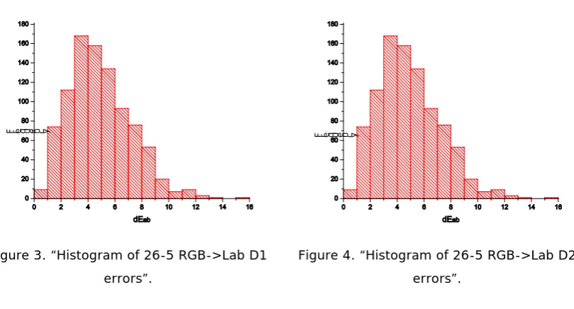
Table 2. “Statistics of the 26-5 model performance”.
JIEM, 2010 – 3(2): 399-407 – Online ISSN: 2013-0953 Print ISSN: 2013-8423
Figure 3. “Histogram of 26-5 RGB->Lab D1 errors”.
Figure 4. “Histogram of 26-5 RGB->Lab D2 errors”.
3.3 Seventh order model with 26 terms
[1 R G B RG GB RB R2 G2 B2 RGB R2G G2B B2R R2B G2R B2G R3 G3 B3 R2GB RG2B
RGB2 R3G2B2 R2G3B2 R2G2B3]
N
∆
E
Min Median Max C.I. 95%RGB->Lab, D1 918 19,63 0,97 16,77 55,56 1,49
RGB->Lab, D2 918 4,94 0,31 4,68 15,88 0,30
Table 3. “Statistics of the 26-7 model performance”.
Figure 5. “Histogram of 26-7 RGB->Lab D1 errors”.
Figure 6. “Histogram of 26-7 RGB->Lab D2 errors”.
F r e q u e n c y F r e q u e n c y
JIEM, 2010 – 3(2): 399-407 – Online ISSN: 2013-0953 Print ISSN: 2013-8423 3.4 Sixth order model with 29 terms
[1 R G B RG GB RB R2 G2 B2 RGB R2G G2B B2R R2B G2R B2G R3 G3 B3 R2GB RG2B
RGB2 R3G2B R2G3B R2GB3 R3GB2 RG3B2 RG2B3]
N
∆
E
Min Median Max C.I. 95%RGB->Lab, D1 918 7,91 0,67 6,56 30,19 0,68
RGB->Lab, D2 918 4,85 0,36 4,54 15,97 0,30
Table 4. “Statistics of the 29-6 model performance”.
Figure 7. “Histogram of 29-6 RGB->Lab D1 errors”.
Figure 8. “Histogram of 29-6 RGB->Lab D2 errors”.
3.5 Seventh order model with 35 terms
[1 R G B RG GB RB R2 G2 B2 RGB R2G G2B B2R R2B G2R B2G R3 G3 B3 R2GB RG2B
RGB2 R3GB RG3B RGB3 R3G2B2 R2G3B2 R2G2B3 R3G2B R2G3B R2GB3 R3GB2 RG3B2 RG2B3]
N
∆
E
Min Median Max C.I. 95%RGB->Lab, D2 918 4,41 0,37 4,18 13,77 0,30
Table 5. “Statistics of the 35-7 model performance”.
JIEM, 2010 – 3(2): 399-407 – Online ISSN: 2013-0953 Print ISSN: 2013-8423
Figure 9. “Histogram of 35-7 RGB->Lab D2 errors”.
As can be seen from Table 1 and Figure 1 and Figure 2, the 23-4 model performed better on the native L*a*b* domain. Adding additional cross product terms and forming more complex models resulted in poorer performance of those models on the native L*a*b* domain. The 26-5 model’s median and mean of errors were increased by ∆E 0,6 and ∆E 0,4 respectively. The maximum error was increased by ∆E 1. The 26-7 model had the worst performance. With the median and the mean of errors of around ∆E 17 and ∆E 20, and the maximum error of around ∆E 56, it is unsuitable for use as the errors are extreme. The 29-6 model also performed worse than simpler models. The median error of ∆E 7, the mean error of ∆E 8, and the maximum error of ∆E 30 are considered to be quite large. On the scaled L*a*b* domain, the performance of the initial 23-6 model was worse than on the native L*a*b* domain. However, more complex models formed by adding additional cross product terms showed better performance, as the median and the mean of errors were reduced. The maximum error was increased. The 26-5 model’s mean and median of errors were reduced by the amount that is not considered to be significant as it falls within the limits of the confidence interval. The maximum error was increased by approximately ∆E 0,7. The 26 -7 model performed similarly. Its mean and median of errors were reduced by insignificant amount, and the maximum error was increased by almost ∆E 1. The 29 -6 model’s mean and the median of errors were reduced by around ∆E 0,2. The maximum error was increased by around ∆E 1.
JIEM, 2010 – 3(2): 399-407 – Online ISSN: 2013-0953 Print ISSN: 2013-8423
errors were reduced by approximately ∆E 0,6, and the maximum error was reduced by around ∆E 1,2. Although it was not tested in this study, it is likely that even more complex models could further improve the accuracy on the scaled L*a*b* domain.
Native L*a*b* Scaled L*a*b*
R,G,B L* a* b* R,G,B L* a* b*
R
ang
e
0 18,38 -47,63 -44,68 0 0,1838 0,315176 0,326745
255 92,11 58,45 69,98 1 0,9211 0,731176 0,776392
Ratio 0,29 0,416 0,45 0,7373 0,416 0,45
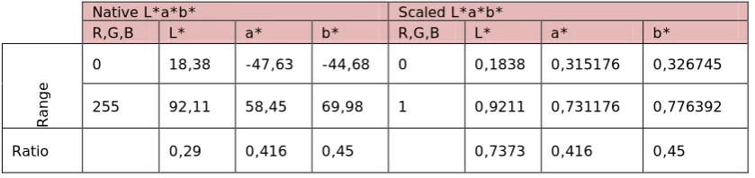
Table 6. “Domain - co domain ratios”.
The polynomial models higher than order fourth over fitted the data on the native L*a*b* domain. On the scaled L*a*b* domain the seventh order model performed well. The data displayed in Table 2 presents the ranges of the data on the two domains, and the ratios of the data ranges on the two domains with respect to their co domains. The purpose of calculating the ratios was to describe the data spread and explain why the over fitting occurs on one domain, and does not occur on the other one. However, the ratios are the same for a* and b* values, and addition test with L* values scaled to produce a ratio of 0,29 gave even better results. The only apparent difference between these two domain lies in the fact that the maximum input values are, in the case of the native L*a*b* domain 255, and in the case of the scaled L*a*b* domain 1. Putting those values under power,
n
x
, in the first case255
n produces large values, while in the second case1
n leaves the value of 1 unchanged. Another consideration that has to be taken into account is that putting values greater than 1 under power produces larger values, while putting values smaller than one produces smaller values than the value under the power. Keeping in mind that there is a positive relationship between the RGB and L* values the results become confusing.4 Conclusion
JIEM, 2010 – 3(2): 399-407 – Online ISSN: 2013-0953 Print ISSN: 2013-8423
from producing different gradients between data points by scaling the data. If the data is fairly linear, the gradient values between pairs of points are similar. Scaling the data by different factors can affect those gradients and make the data less linear. However, in this case, both domain and co domain values were scaled by the same factor, leaving the gradients unchanged. The fact that putting value smaller than 1 under the power produces a value smaller than the value under the power produced better results when modeling variables with positive relationship can be explained by simple adaptation of the estimated coefficients to model this relationship. Aside from the obvious difference of the behavior of maximum values 255 or 1 under the power, it was noted that by scaling the L* value by 255 produced better results than scaling it by 100. This effect should be further studied and tested on other, a* and b* values as well as it appears to have a potential for further improvements.
References
Croarkin, C., Tobias., P. et al. (2003). Engineering Statistics Handbook. Retrieved
August 13th, 2010, from
Chou, Y.-F. (2010, June). Digital Camera Calibration Target Selection With Different Materials. Paper presented at Create 2010 Conference, Gjovik, Norway.
Green, P., & MacDonald, L. (2002). Colour Engineering. Chichester: Wiley
Sharma, G. et al. (2003). Digital Color Imaging Handbook. Boca Raton: CRC Press.
Specification ICC.1:2004-10. ICC
Thomas, J.B. (2010, June). Controlling Color in Display: A Discussion on Quality. Paper presented at Create 2010 Conference, Gjovik, Norway.
©© Journal of Industrial Engineering and Management, 2010
Article's contents are provided on a Attribution-Non Commercial 3.0 Creative commons license. Readers are allowed to copy, distribute and communicate article's contents, provided the author's and Journal of Industrial Engineering and Management's names are included. It must not be used for commercial purposes. To see the complete