Standardisation of eddy-covariance flux measurements of methane and nitrous oxide

Standardisation of eddy-covariance flux measurements of methane and nitrous oxide

Giacomo Nicolini18_{, Mats B. Nilsson}19_{, Olli Peltola}2_{, Janne Rinne}14_{, and Mark Zahniser}17 1_{Centre for Ecology and Hydrology, Bush Estate, Penicuik, EH26 0QB, UK}

2_{Institute for Atmospheric and Earth System Research/Physics, Faculty of Science, P.O. Box 68, FI-00014 University of Helsinki, Finland} 3_{Department of Environmental Engineering, Technical University of Denmark, Bygningstorvet, 2800 Kgs. Lyngby, Denmark} 4_{Finnish Meteorological Institute, P.O. Box 503, 00101, Helsinki, Finland}

5_{R&D, LI-COR Biosciences, Lincoln, Nebraska, NE 68504, USA}

6_{Bio-Atmospheric Sciences, University of Nebraska, Lincoln, Nebraska, NE 68508, USA}

7_{Climate Sciences, Lawrence Berkeley National Laboratory, One Cyclotron Rd, Berkeley, CA, 94720, USA} 8_{Research Centre of Excellence Plants and Ecosystems (PLECO), University of Antwerp, Wilrijk, Belgium} 9_{Department of Ecology, Swedish University of Agricultural Sciences, SE-750 07 Uppsala, Sweden}

10_{TERRA Teaching and Research Centre, Gembloux Agro-Bio Tech, 33 University of Liege, B-5030, Gembloux, Belgium} 11_{Zentrum für Agrarmeteorologische Forschung Braunschweig (ZAMF), Deutscher Wetterdienst, Bundesallee 50,} 38116, Braunschweig, Germany

12_{Department of Environmental Systems Science, Institute of Agricultural Sciences, ETH Zurich, Universitätstrasse 2,} 8092 Zürich, Switzerland

13_{Department of Earth Sciences, University of Gothenburg, P-O. Box 460, SE 405 30 Gothenburg, Sweden}

14_{Department of Physical Geography and Ecosystem Science, Lund University, Sölvegatan 12, 22362 Lund, Sweden} 15_{Agronomy and Horticulture, University of Nebraska, Lincoln, NE 68508, USA}

16_{Mazingira Centre, International Livestock Research Institute (ILRI), P.O. Box 30709, 00100 Nairobi, Kenya} 17_{Aerodyne Research, Inc., 45 Manning Road, Billerica, MA, USA 01821-3976}

18_{Department for Innovation in Biological Agro-food and Forest systems, University of Tuscia, Via San Camillo de Lellis,} 01100 Viterbo, Italy

19_{Department of Forest Ecology and Management, Swedish University of Agricultural Sciences, SE-116 90183, Umeå, Sweden}

Received March 16, 2018; accepted August 27, 2018

*Corresponding author e-mail: en@ceh.ac.uk

A b s t r a c t. Commercially available fast-response analysers for methane (CH4) and nitrous oxide (N2O) have recently become more sensitive, more robust and easier to operate. This has made their application for long-term flux measurements with the eddy- covariance method more feasible. Unlike for carbon dioxide (CO2) and water vapour (H2O), there have so far been no guidelines on how to optimise and standardise the measurements. This paper reviews the state-of-the-art of the various steps of the measure-ments and discusses aspects such as instrument selection, setup and maintenance, data processing as well as the additional meas-urements needed to aid interpretation and gap-filling. It presents the methodological protocol for eddy covariance measurements

of CH4 and N2O fluxes as agreed for the ecosystem station net-work of the pan-European Research Infrastructure Integrated Carbon Observation System and provides a first international standard that is suggested to be adopted more widely. Fluxes can be episodic and the processes controlling the fluxes are complex, preventing simple mechanistic gap-filling strategies. Fluxes are often near or below the detection limit, requiring additional care during data processing. The protocol sets out the best practice for these conditions to avoid biasing the results and long-term budg-ets. It summarises the current approach to gap-filling.

K e y w o r d s: ICOS, protocol, micrometeorology, greenhouse gas exchange, standardisation

INTRODUCTION

Methane (CH4) and nitrous oxide (N2O) are the second

and third most important greenhouse gases after carbon dioxide (CO2). Methane has a lifetime of about 12.4 years

and a global warming potential (GWP) of 34 (over the 100-year horizon), whilst N2O has a lifetime of about 121 years,

with a GWP of 298 (IPCC, 2013). As a result, although

their fluxes tend to be considerably smaller than that of

CO2, they often significantly alter the net greenhouse gas

balance of terrestrial and aquatic systems with the

atmos-phere. Because concentrations and fluxes of these non-CO2

greenhouse gases (GHGs) are smaller than those of CO2,

this imposes additional challenges for the instrumentation used for their measurement and data processing.

Instrumentation has been available for more than three

decades to make eddy-covariance (EC) flux measurements of

CO2 and water vapour (H2O), that is reliable and reasonably

affordable in terms of purchase and operation. As a re-

sult of this, and also reflecting the importance of CO2,

flu-xes of CO2 are measured across large regional networks

and significant effort has gone into the harmonisation of

approaches and development of best practices (Aubinet et

al., 2000, 2012).

By contrast, the first EC flux measurements of CH4

and N2O were not made until the 1990s and initially with

tunable diode laser absorption spectrometers that had rela-tively high noise levels and required regular cooling with

liquid nitrogen and were difficult to maintain long-term.

Fast response analysers for measuring CH4 and N2O flux

-es that are easy-to-deploy in the field have only become

available during the past decade. As a result, the num-ber of existing long-term measurements and experience in instrument setup, instrument long-term performance,

data processing and evaluation of non-CO2 flux estimates

remains comparatively limited and approaches have not yet been standardised. This is further exacerbated by the limited success of reproducing the underlying biogeochem-ical processes of CH4 and in particular N2O exchange with

simple empirical relationships (for more details please see Butterbach-Bahl et al., 2013; Eugster and Merbold, 2015). Because older instrumentation could only detect relatively

large fluxes and even the more recent instrumentation is deployed to target the largest fluxes, much of the current

experience is based on so-called high-emission ecosys-tems, e.g. CH4 emissions from wetlands and N2O emissions

in agricultural fields. An overview of studies that focused on EC flux measurements of CH4 and/or N2O is given in

Table 1, with particular emphasis on studies more recent than the overview of EC results up to 2012 provided by Nicolini et al. (2013).

With the latest generation of analysers it is now possible to measure CH4 and N2O fluxes near their background lev

-el, which can still add up to a considerable fraction of the

annual budget. Still significantly more expensive than com

-parable sensors for CO2, the newer instruments are much

more stable and cost-efficient to operate, and no longer

require continuous cooling with liquid nitrogen, a major

challenge in field applications. This makes them increas -ingly deployable across large-scale networks such as the Integrated Carbon Observation System (ICOS), a pan- European research infrastructure (as described in the intro-ductory paper to this issue), and the National Ecological Observatory Network (NEON) in the US. Within ICOS,

EC flux measurements of CH4 and N2O are mandatory for

all Class-1 Stations (ibid.) and further recommended for

Class-2 Stations, but only if CH4 and N2O fluxes are rel

-evant to the overall GHG budget of the site. Guidelines on the relevance criteria are given below.

This paper provides a first step towards a best practice

in the set-up and data processing associated with measuring

EC fluxes of CH4 and N2O, focusing on those

considera-tions that are additional or different to those for making CO2 flux measurements, where one reoccurring issue is

the measurement of fluxes close to the limit of detection

(LOD) of the instruments. Besides the measurements of CH4 and N2O, it is crucial to complement GHG flux

measurements with specific ancillary data. Such data are important for two reasons: (1) to explain measured flux

values and thereby generate additional knowledge about which variables drive the underlying processes and (2) to provide ancillary variables that may be crucial for

poten-tial gap-filling approaches. Gap-filling can be done with

simple averaging methods, leading to large uncertainties

or with more complex approaches, including artificial

neural networks, multiple imputation techniques, as well

as process-based biogeochemical models. Yet, gap-filling

of discontinuous measurements is crucial to derive the full GHG budget of a site.

One key difference that distinguishes fluxes of CH4 and

N2O from those of CO2 is that the CO2 flux tends to be

strongly bi-directional over the diurnal cycle and that the annual budget for ecosystems tends to be a small difference between a large downward component during the day and a large upward component during the night, which makes it particularly important to quantify both components

cor-rectly. The flux of N2O tends to be upward for most of

the time (the uptake rates are generally so low that they will be within the noise level), whilst for CH4 both uptake

(oxidation) and emission are observed, but changes typi-cally occur between sites or seasons, rather than following a diurnal cycle. Thus, the annual budget of CH4 and N2O

is much less sensitive to the accuracy of corrections that preferentially apply during day or night-time. By contrast, for N2O in particular, the flux can be highly episodic, and

during a few days (Zona et al., 2013a, 2013b; Zenone et al., 2016), e.g. related to fertiliser applications, rain episodes or freeze-thaw cycles (Matzner and Borken, 2008; Groffman

et al., 2009; Molodovskaya et al., 2012; Wagner-Riddle et al., 2017). As a result, unlike chamber approaches, the EC method is ideally suited for capturing the high emission events with good spatial representativeness and temporal

coverage, but it may well be challenged by the small fluxes

during the remainder of the year.

Open-path measurements of CH4 and other gases with

fluxes relatively small in comparison to their typical atmos -pheric concentrations are subject to large correction terms

for density fluctuations caused by fluxes of sensible and

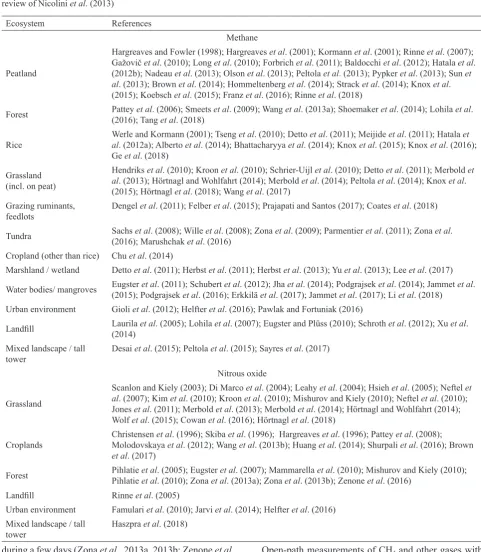
latent heat (referred to as the WPL correction; Webb et al., 1980), the uncertainty of which dominates the effective detection limit of these instruments. For this reason, and because of data loss by precipitation, open-path sensors for CH4 are not accepted for ICOS ecosystem Class 1 Stations. Table 1. Overview of selected existing eddy-covariance studies on CH4 and N2O exchange, with focus on those published since the review of Nicolini et al. (2013)

Ecosystem References

Methane

Peatland

Hargreaves and Fowler (1998); Hargreaves et al. (2001); Kormann et al. (2001); Rinne et al. (2007); Gažovič et al. (2010); Long et al. (2010); Forbrich et al. (2011); Baldocchi et al. (2012); Hatala et al. (2012b); Nadeau et al. (2013); Olson et al. (2013); Peltola et al. (2013); Pypker et al. (2013); Sun et al. (2013); Brown et al. (2014); Hommeltenberg et al. (2014); Strack et al. (2014); Knox et al. (2015); Koebsch et al. (2015); Franz et al. (2016); Rinne et al. (2018)

Forest Pattey _{(2016); Tang} et al. (2006); Smeets _{et al. (2018)} et al. (2009); Wang et al. (2013a); Shoemaker et al. (2014); Lohila et al.

Rice Werle and Kormann (2001); Tseng al. (2012a); Alberto et al. (2014); Bhattacharyya et al. (2010); Detto et al. (2014); Knox et al. (2011); Meijide et al. (2015); Knox et al. (2011); Hatala et al. (2016); et Ge et al. (2018)

Grassland (incl. on peat)

Hendriks et al. (2010); Kroon et al. (2010); Schrier-Uijl et al. (2010); Detto et al. (2011); Merbold et al. (2013); Hörtnagl and Wohlfahrt (2014); Merbold et al. (2014); Peltola et al. (2014); Knox et al. (2015); Hörtnagl et al. (2018); Wang et al. (2017)

Grazing ruminants,

feedlots Dengel et al. (2011); Felber et al. (2015); Prajapati and Santos (2017); Coates et al. (2018)

Tundra Sachs _{(2016); Marushchak} et al. (2008); Wille _{et al. (2016)}et al. (2008); Zona et al. (2009); Parmentier et al. (2011); Zona et al. Cropland (other than rice) Chu et al. (2014)

Marshland / wetland Detto et al. (2011); Herbst et al. (2011); Herbst et al. (2013); Yu et al. (2013); Lee et al. (2017)

Water bodies/ mangroves Eugster _{(2015); Podgrajsek} et al. (2011); Schubert _{et al. (2016); Erkkilä} et al. (2012); Jha _{et al. (2017); Jammet} et al. (2014); Podgrajsek _{et al. (2017); Li} et al. (2014); Jammet _{et al. (2018)} et al. Urban environment Gioli et al. (2012); Helfter et al. (2016); Pawlak and Fortuniak (2016)

Landfill Laurila ₍₂₀₁₄₎ et al. (2005); Lohila et al. (2007); Eugster and Plüss (2010); Schroth et al. (2012); Xu et al. Mixed landscape / tall

tower Desai et al. (2015); Peltola et al. (2015); Sayres et al. (2017) Nitrous oxide

Grassland

Scanlon and Kiely (2003); Di Marco et al. (2004); Leahy et al. (2004); Hsieh et al. (2005); Neftel et al. (2007); Kim et al. (2010); Kroon et al. (2010); Mishurov and Kiely (2010); Neftel et al. (2010); Jones et al. (2011); Merbold et al. (2013); Merbold et al. (2014); Hörtnagl and Wohlfahrt (2014); Wolf et al. (2015); Cowan et al. (2016); Hörtnagl et al. (2018)

Croplands Christensen Molodovskaya et alet al. (1996); Skiba . (2012); Wang et alet al. (1996); Hargreaves . (2013b); Huang et alet al. (2014); Shurpali . (1996); Pattey et alet al. (2008); . (2016); Brown et al. (2017)

Forest Pihlatie _{Pihlatie et al}et al. (2005); Eugster _{. (2010); Zona et al}et al_{. (2013a); Zona} . (2007); Mammarella _{et al. (2013b); Zenone} et al. (2010); Mishurov and Kiely (2010); _{et al. (2016)}

Landfill Rinne et al. (2005)

Urban environment Famulari et al. (2010); Jarvi et al. (2014); Helfter et al. (2016) Mixed landscape / tall

Nevertheless, they may be appropriate in some situations and may be the only option for the remote and low-power installations (Appendix 1 on how to minimise errors in the WPL correction through care in setup, operation and pro-cessing of the measurements of all components). Whilst open-path analysers are not yet commercially available

for N2O, developments are underway to reduce pumping

requirements for closed-path systems (Brown et al., 2017). In general, the ICOS methodology will further develop over time, by reformulating measurement requirements according to the experiences and implementation of new technological achievements. This is particularly true for

this protocol on EC flux measurements of CH4 and N2O

because it seeks to develop the first international standard

of its kind. Analysers and experience with their long-term operation are currently developing at speed.

In this paper, we aim to provide guidelines for EC flux

measurements of CH4 and N2O, and state for which

eco-system types either measurement is feasible, together with guidelines for selecting instruments that are capable of

measuring these non-CO2 GHG fluxes. We further provide

recommendations on the setup of EC flux measurements,

maintenance and calibration intervals as well as a list of recommended ancillary variables that should be measured. At the end of this paper, we highlight crucial steps that need to be undertaken when processing CH4 and N2O flux data,

which quality criteria should be applied and how potential

gaps in data could be filled.

Throughout the paper the focus is on those aspects that need to be considered additionally when making and interpreting EC measurements of CH4 and N2O, besides the

aspects that are covered by energy and CO2 flux measure

-ments already (see protocols for ICOS flux station setup and

EC data processing in this issue).

METHODOLOGY

Instrument sensitivity and ecosystem applicability Measurement method

At the time of writing, all fast response analysers for

CH4 and N2O available are based on a range of optical

absorption techniques. Methane flux measurements have also been made with a flame ionisation detector (FID) (Fan et al., 1992; Laurila et al., 2005; Lohila et al., 2007), but this approach is sensitive also to non-methane hydrocarbons

and thus not sufficiently specific for general application in

an EC setup. Of the closed-path instruments based on opti-cal absorption techniques, most (with the exception of the

Campbell Scientific TGA) use multi-pass cells and include

tunable infrared laser differential absorption spectrometers

(TILDAS) (e.g. Aerodyne Res. Inc.; Campbell Scientific),

cavity ring-down spectrometers (CRDS; e.g. Picarro Res.

Inc.) and off-axis integrated cavity output spectroscopy (Los Gatos Research, LGR). These may deploy lead-salt

lasers (older instruments), telecom lasers (CH4 only) or

quantum cascade lasers and typically target CH4 and N2O

on absorption features in the mid-infrared range. Depending on the exact absorption features (wavelength range) used, the same instruments may measure several compounds at the same time, e.g. CH4 only, CH4/CO2, N2O/CH4, N2O/

CO2, N2O/CO. Most current instruments also derive H2O

mole fraction, which is needed for internal corrections, while some legacy instruments and the current TGA200A

(Campbell Scientific) do not. With absorption features

differing in intensity, the different options target CH4 and

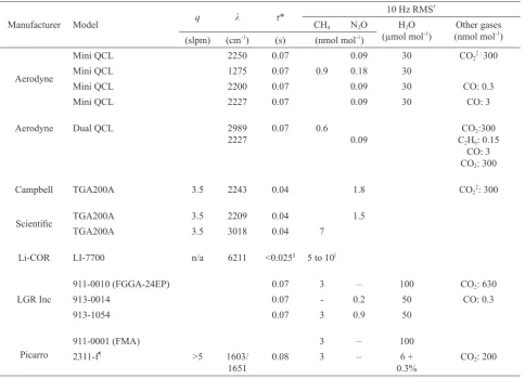
N2O with varying sensitivity. Table 2 compiles the

instru-ments known to be available at the time of writing, together

with their specifications, bearing in mind that this is a fast-moving field. Other commercial instruments exist, but have not been demonstrated to be sufficiently fast for EC flux

measurements. In addition to the closed-path sensors, the LI-COR LI-7700 is currently the only commercial open-path sensor available. Based on wavelength modulation

technology it targets CH4 only. Similar non-commercial

open and closed-path flux instruments exist in a number of

research laboratories and universities. Measured quantities

The key measurement for the calculation of EC fluxes

is a highly time-resolved measurement of N2O and/or CH4.

A scalar intensity of an atmospheric constituent s may be described by several metrics (ISO80000-9:2009(E)) (ISO, 2009): “mass concentration (ρs, kg m-3)” or

“concentra-tion (cs, mol m-3_{)” representing the mass or the amount of}

substance of s per volume of air, respectively. The “mass fraction (kg kg-1_{)” is the ratio of the mass of s divided by}

the mass of the mixture, whilst the “mole fraction (χs, mol mol-1_{)” is the ratio of the amount of substance of s divided}

by the totalamount of substance of the mixture (also equal to the ratio of the constituent partial pressure to the total pressure). The “dry mole fraction (χsd, mol mol-1_{)” is the}

ratio of the amount of substance of s to that of dry air. These variables are related by the ideal gas law and the Dalton law. Conversion factors are given in Table 3.

Amongst these variables, only the dry mole fraction is a conserved quantity of the substance in the presence

of changes in temperature, pressure and H2O content

(Kowalski and Serrano-Ortiz, 2007). Unfortunately, gas analysers based on optical spectroscopy techniques measure absorption, which is directly related to (molar) concentration – a metric that is not conserved in these con-ditions. Therefore, concentration variations may appear in the absence of production, absorption or transport of the

component. For this reason, the turbulent flux, that is rep -resentative of the ecosystem source/sink intensity, is the covariance of the vertical wind velocity and the component dry mole fraction.

A number of disparate flux units are in use in the com

-munity that measures fluxes of CH4 and N2O. Having

Table 2. Manufacturer-provided characteristics of commercially available fast-response gas analysers for CH4 and N2O. q is the flow rate through the instrument cell, λ indicates the approximate wavelength (expressed as wave number) of the absorption features used, whilst τ is the time response of the instrument itself as stated by the manufacturer, if the pump recommended for fast-response instru-ments is used

Manufacturer Model q λ τ*

10 Hz RMS†

CH4 N2O H2O

(µmol mol-1_{) (nmol mol}Other gases-1₎ (slpm) (cm-1_{) (s) (nmol mol}-1₎

Aerodyne

Mini QCL 2250 0.07 0.09 30 CO2‡ : ₃₀₀

Mini QCL 1275 0.07 0.9 0.18 30

Mini QCL 2200 0.07 0.09 30 CO: 0.3

Mini QCL 2227 0.07 0.09 30 CO: 3

Aerodyne Dual QCL 2989

2227 0.07 0.6 0.09 C2H6: 0.15CO2:300

CO: 3 CO2: 300

Campbell TGA200A 3.5 2243 0.04 1.8 CO2‡_{: 300}

Scientific TGA200A 3.5 2209 0.04 1.5

TGA200A 3.5 3018 0.04 7

Li-COR LI-7700 n/a 6211 <0.025§ _{5 to 10}||

LGR Inc

911-0010 (FGGA-24EP) 0.07 3 – 100 CO2: 630

913-0014 0.07 - 0.2 50 CO: 0.3

913-1054 0.07 3 0.9 50

Picarro

911-0001 (FMA) 3 – 100

2311-f¶ _{>5 1603/}

1651 0.08 3 – 0.3%6 + CO2: 200

*Flow response time with recommended appropriate (external) high flow vacuum pump; †typically calculated as the Allan Deviation with 0.1 s averaging time; where only 1 Hz values were available, these have been multiplied by √10. ‡Scaled up from 13_CO2; §_the effective ability to resolve eddies is limited by wind speed and spatial eddy averaging; ||_{5 ppb at 10 Hz when instrument is clean; 10 ppb} at 10 Hz when instrument is dirty (RSSI 20%); flux uncertainty is dominated by additional uncertainty in the WPL terms; ¶_{precision is} for 3-species mode (CO2/CH4/H2O) operation.

Table 3. Conversion factors between some variables describing the scalar intensity of an atmospheric constituent

Conversion factor Dry mole fraction (nmol mol-1₎ csd =

Concentration (nmol m-3₎

cs =

Mass concentration (ng m-3₎

ρs = Dry mole fraction

csd × 1

−

a v a

p p

RT ( )

−

s a v a

m p p RT

Concentration

cs × a−av

RT

p p 1 ms

Mass concentration

ρs × s( a−a v)

RT

m p p m1_s 1

The variable in the column header is obtained by multiplying the variable in the line header by the factor given in the table; pa: atmos-pheric pressure (Pa); pv: water vapour pressure (Pa); R: gas constant (8.314 J K-1 _mol-1_{); Ta: air temperature (K); m}

closed for about one hour, hourly flux units are quite com -mon. However, for consistency between compounds and to follow SI standards, it is recommended to use nmol m-2 _s-1

for individual flux values, whilst annual budgets should be

expressed in g CH4-C m-2 y-1 and kg N2O-N ha-1 y-1. The

latter enables easy comparison of CH4 fluxes with those of

CO2 and quantification of N2O losses in relation to fertiliser

input and atmospheric N deposition, both of which are usu-ally expressed in kg N ha-1 _y-1_.

Criteria for analyser selection and minimum annual budgets to be resolved

The issue of analyser selection is closely linked to the question about the stations for which the EC CH4 and N2O

flux measurement is recommended, based on the relevance

and contribution of CH4 and N2O fluxes to the site-based

greenhouse gas balance. For ICOS ecosystem Class 1

Stations, flux measurements of CH4 and N2O by both EC

and automated chamber methods are required, unless it is demonstrated (e.g. by means of short-term campaigns) that

these fluxes are not relevant for the site. As an example,

a station that does not measure N2O fluxes would be eligi

-ble of being a Class 1 Station, if it can be proven that N2O

fluxes are negligibly small for that site, e.g. by means of shorter-term manual chamber campaigns. Up to now, “not

relevant” and “negligibly small” were still to be defined.

We recommend that for the application of EC methods to CH4 and N2O the following criteria should be considered:

1. The detection limit of current gas analysers: here the basis should not be the performance of the most sensitive analyser under laboratory conditions, but the reasonably

maintainable performance of the latest generation of flux analysers that can be expected under field conditions. The quantification of the precision should include the addi -tional uncertainty introduced by the conversion to dry mole fraction.

2. The relative contribution of the CH4 and N2O flux to

the total atmospheric GHG budget at the site.

3. The relevance of the magnitude of the fluxes from

the ecosystem type to the global terrestrial CH4 and N2O

budgets.

4. Comparative merits with the alternative chamber method.

The random flux error and therefore the flux detection

limit is determined by instrument noise (and its interplay with turbulence) as well as by random geophysical variabil-ity. Whilst for CO2 the latter dominates in most conditions,

this is not necessarily true for CH4 and N2O. Thus, the flux

detection limit depends on the precision of the concen-tration measurement, but also on the turbulence and site characteristics. The random error due to instrument noise can be approximated as (Mauder et al., 2013):

(1)

where: is the instrument noise, σw is the standard

deviation of the vertical wind component and N is the

number of (e.g. 10-Hz) data points the flux calculation is

based on (typically 18000 for a 30-min averaging period of 10-Hz data).

For N2O it is estimated that an annual flux of 0.5 kg

N2O-N ha-1 y-1 is quantifiable by EC using the latest genera

-tion of QCL based instruments. Assuming a situa-tion where 80% of the annual emission occurs during 2 weeks, the ave-

rage background flux during the remainder of the year would

then equate to 0.024 nmol m-2 _s-1_{, whilst the average flux}

during the high emission period would be 2.4 nmol m-2 _s-1_.

This estimate comes from the first available long-term flux measurement datasets from managed crops and grass -land measured with this technology (e.g. Huang et al., 2014; as well as unpublished datasets obtained by the authors; Merbold et al., 2014) and is also consistent with the

detec-tion limit reported during field deployments. Based on an

intercomparison study carried out during the Integrated

non-CO2 Greenhouse gas Observing System (InGOS)

pro-ject, Nemitz et al. (2018) reported differences in standard

deviations of flux values derived in the field were about

twice the value reported by the manufacturers. A real-world precision of 1 nmol mol-1 _{is maintainable by several}

current-ly available N2O instruments (Rannik et al., 2015; Nemitz et al., 2019). Given a typical range of u* values of 0.15 to

1 m s-1 _{and a ratio of σw/u}

* = 1.29 under neutral conditions,

this u* range equates to a limit of detection due to

instru-ment noise (LOD = 3 x relative error (RE)) of 0.20 to 0.84 nmol m-2 _s-1_{. This is clearly adequate for quantifying the}

N2O flux estimated during high flux periods. In addition, if

care is taken in the setup, operation and processing of the

data, REs become smaller if small flux measurements are averaged according to time or another parameter, by 1/√n,

where n is the number of 30-min fluxes that are being aver -aged (Langford et al., 2015). Thus, the detection limit of

the estimated background flux is approached for averaging

periods of 1.4 to 25.5 days, depending on u*, and certainly

for monthly values. To achieve this an RMS of 1 nmol mol-1

needs to be maintained under field conditions.

For CH4, fluxes tend to have a less episodic annual pat

-tern than those of N2O. To evaluate which magnitude may

be relevant at the global scale, the average global wetland

CH4 emission can, as an example, be estimated from the

global CH4 emission (200 Tg CH4 y-1; IPCC (2013)) and

wetland area (5×1012 _m2_{; Matthews and Fung (1987)) as 34 g}

CH4-C y-1 (equivalent to 90 nmol m-2 s-1). Nevertheless,

a low flux that is still deemed relevant at the global scale is the winter emission background flux from northern

wetlands, which is typically around 7 nmol m-2 _s-1

(equiva-lent to 2.6 g CH4-C m-2 y-1) (Rinne et al., 2007). To achieve

precision needs to be in the range 8 to 35 ppb, depending on u*. Indeed, a real-world precision of 10 ppb is

attain-able by several instruments. Thus, EC measurements are deemed suitable to measure annual emission budgets of 2.5 g CH4-C m-2 y-1 and for this real-world analyser a

preci-sion of at least 10 nmol mol-1 _{needs to be maintained.}

Other instrument criteria

In addition to these criteria, the gas analyser must have an internal water measurement for water corrections to be applied accurately. Most commercially available closed-path instruments now correct for H2O and provide dry mole

fraction of CH4 and N2O. Some of the older instruments

that do not report H2O can be upgraded at reasonable cost.

The TGA200A of Campbell Scientific does not provide an

internal H2O measurement and therefore does not meet the

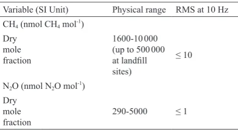
requirements of ICOS Class 1 stations. The instruments should be capable of measuring over the concentration ranges summarised in Table 4.

The analyser should further a priori be capable of pro-viding high data capture of, e.g., >90%, and any data gaps should be uncorrelated with meteorology. Thus, the planned use of the analyser for calibrations, performance tests etc. should not exceed 10% of the time nor occur during

poten-tial high flux periods. As will become apparent later in this

protocol, the data processing and quality control for small

fluxes is greatly facilitated if the instruments also measure larger fluxes of another compound. Thus, in particular for

N2O, for which fluxes can be small for extensive periods,

it helps greatly to use a combined N2O-CO2 instrument.

However, where CO or CH4 fluxes are consistently large,

combined N2O-CO and N2O-CH4 analysers, respectively,

can similarly facilitate the data analysis.

At the time of writing only closed-path analysers fulfil

the requirements set out above.

Instrument setup for closed-path analyser eddy covariance systems

Closed-path sensors are currently the only choice for building a non-CO2 GHG EC system that fulfils the require

-ments set out in the previous section. Through the setup of the closed-path analyser, high-frequency concentration attenuation takes place. It is the goal of this section to describe a setup of such an EC system that minimises the

high-frequency flux losses as efficiently as possible for long-term flux applications.

Although analysers listed in Table 2 are capable of mea-suring gas concentrations with a temporal resolution of up to 10 Hz, several reasons like air mixing through the gas sampling system and/or the separation between sample air inlet and the centre of the sonic anemometer’s transducer

array usually lead to attenuation of high-frequency fluctua -tions and time delays between the concentration signal and the wind measurement. A robust setup seeks to minimise

the flux loss, whilst, at the same time, trying to establish

the predictable behaviour of the system that allows cor-rection with automated standard methods (see below). For this, the spectral attenuation caused by the sampling

sys-tem configuration needs to be determined and kept in an

acceptable range under long-term use. A maximum of 30% correction compared to a reference model spectrum under neutral conditions is acceptable. This requirement needs to be guaranteed through the interaction and relation of

sys-tem parameters such as pump size, flow rate, tube diameter

(which jointly dictate the Reynolds number), inlet

mount-ing position, filter dimensions etc.

Relative position of the tube inlet and the sonic path

The current closed-path, non-CO2 GHG analysers are

sensitive to temperature fluctuations in the environment

and are relatively bulky. This is why, unlike CO2/H2O

sen-sors, they can generally not be placed on a tower. Thus,

compared with the recommended ICOS CO2/H2O analyser

setup which is described in a companion paper of this issue,

closed-path non-CO2 GHG EC systems have inevitably

longer inlet tubes. Current closed-path laser devices have

voluminous sample cells that require a large sampling flow,

and the usually low pressure in the sample cell requires powerful pumps. Altogether, this makes the task of reduc-ing the high-frequency dampreduc-ing of an EC system much

more challenging compared with the CO2/H2O EC system.

The position of the inlet represents a compromise: it should be as close as possible to the sonic path while minimising perturbations of the micro-turbulence between the sonic transducers. The relative position also affects the system’s time response. Different parameterisations of transfer functions suggest that the system cut-off frequency may depend on various factors such as lateral separation between sensors, atmospheric stability, wind velocity and direction that have been described by Moore (1986),

Kristensen et al. (1997), and Horst and Lenschow (2009).

Table 4. Measured variables, their units, physical range and re- quired precision

Variable (SI Unit) Physical range RMS at 10 Hz CH4 (nmol CH4 mol-1₎

Dry mole fraction

1600-10 000 (up to 500 000 at landfill sites)

≤ 10

N2O (nmol N2O mol-1₎ Dry

mole

If good practice is followed, inlet characteristics can be achieved that capture most of the frequencies that carry the

vertical flux, given that a relatively small flux component

is carried by frequencies > 5 Hz for most wind velocity conditions (Moore, 1986). The ICOS guidance is to share the position of the inlet of the IRGA, with the default sam-pling point being the end of the horizontal boom of the Gill HS ultrasonic anemometer as outlined in the protocol for

the ICOS flux station setup of this issue. If the inlet flow

for the N2O/CH4 analyser(s) is particularly high (> 20 lpm),

it may be more appropriate to increase horizontal displace-ment by another 10 cm or so. The inlet should be kept as compact as possible.

Features of the gas sampling system

The sample air is transported through the gas sampling system to the analyser cell. Generally, a number of princi-ples have to be considered to operate a system that ensures gas concentration measurements of highest possible quali-ty. These principles – though being hardly compatible – are a minimisation of:

• the high-frequency attenuation of the concentration mea- surement,

• the cell contaminations with particles,

• pump-induced pressure fluctuations,

• air flow perturbation around the anemometer head caused

by the tube,

• large temperature differences between the air sample and the instrument’s optics that could lead to erroneous ana-lyser readings,

• H2O effects on sample concentration, • temperature fluctuations of the analyser.

To meet the constraints outlined above, adjustments

to pump, tube, filter, temperature-controlled housing, etc. have to be made and are described in the following sections.

Inlet dryer

It is a requirement for the gas analyser to measure H2O

internally so that accurate corrections can be performed. An additional inlet dryer adds complexity and can dete-riorate the system response time, so is not generally

recommended. However, where non-CO2 fluxes are very

small and latent heat fluxes large, such dryers can be used as an option to improve the flux detection limit (see Results

and Discussion below) and need not remove 100% of the H2O to improve the flux detection limit. In such situation,

a high-flow Nafion dryer can be used, which can be pumped

by the same vacuum pump used for the measurement cell. Here, the integrity of the dryer needs to be monitored

con-tinuously through the internal H2O measurement.

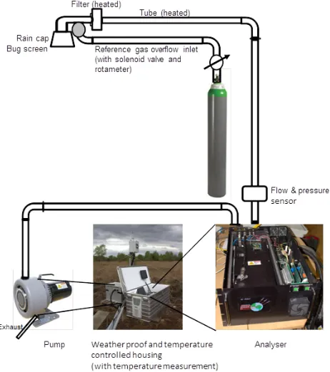
General layout, pump and system dimensioning From upstream to downstream, the gas sampling system

consists of a rain cap with bug screen, an overflow solenoid valve to provide a reference gas (reference gas overflow

inlet, RGOI), a filter or set of filters, a sampling tube, the dryer (if present, see previous section), a flow and pressure sensor, the gas analyser, possibly another filter, and a pump.

After passing the pump, the sample air is returned to the

outside air through an exhaust (Fig. 1). Rain cap, filter and

tube induce a pressure drop depending on their characte-

ristics and on the flow rate. However, most analysers only

operate over a limited pressure range. The user has to make

sure that rain cap, filter, and tube fulfil the specifications

given below and the given pressure regime. For current instruments, drying of the air sample is not required.

Furthermore, dimensioning of the sampling system and

pump has to meet the following specification:

• The gas filling the sampling cell under operation should

at least be exchanged 10 times per seconds, i.e. the cell turn-over time (τcell) should be < 100 ms.

• A filter and tube cut-off frequency should be as high as

possible (ideally above 10 Hz). This also implies that the

flow must be turbulent in all sections of the inlet. The guiding principle here is that maximum flux attenuation

under neutral conditions of the entire sampling system (incl. analyser) should not exceed 30%.

Reference gas overflow inlet (RGOI)

A normally-closed solenoid valve (or similar) needs to be installed at/near the tube inlet for a reference gas, through which a reference gas can be injected into the inlet

via a T-piece, at a flow just higher than the regular sample flow at regular intervals (see section on instrument calibra -tion below). This reference gas should be of a concentra-tion

distinct of the ambient concentration, but well within the range of the analyser. This can either be an elevated mix-ture of CH4 and/or N2O in air or N2 (e.g. at roughly 2500

and 500 ppb, respectively) and, as long as it fulfils these

requirements, the mixture does not need to be calibrated

or certified. Alternatively, in many cases a cheap industrial

compressed air cylinder can be found that contains slightly

elevated concentrations. The flow through the solenoid

inlet should be adjusted (e.g.via a rotameter) to be just (e.g. 10%) above the highest flow rate expected through the inlet.

Care needs to be taken that, when activated, the sample line

pressure is close to normal to avoid pressure fluctuations in

the analyser. The reference gas should be applied for 5-min, to assess the inlet response time and time-lag every three days (see below). It should further be activated for a 30-min period at least every month to assess the instrument stabil-ity in terms of instrumental noise and low-frequency drifts.

For a system running at 15 lpm with this scheme a 10 m3

cylinder will last for just over 8 months. Pump

The pump must be strong enough to provide the

desig-nated flow rate in order to maintain at least 10 cell renewals

per second. The cell turn-over time (τcell) for a given flow can be estimated as:

τcell = Vcell / qinlet pcell / p0, ₍₂₎

where: Vcell is the cell volume (cm3_{), qinlet is the inlet mass}

flow in standard cm3 _s-1_{, and pcell and p}

0 are cell and standard

(101.25 kPa) pressure, respectively. This τcell is equivalent to the e-folding time of the system and thus describes a 63% response. The 95% response time (τ95) is three times longer.

Pump capacity must significantly exceed the nominal flow

rate selected for the system to lengthen pump longevity and to establish low pressures in the cell. If the cell volume is for example 0.5 L and the cell pressure ~40 Torr as is the case for Aerodyne’s mini-QCL (Aerodyne Research Inc.

Billerica, MA, USA), this implies that the flow rate has to

be adjusted to at least 12-15 standard L min−1_.

Robustness and durability of the pump are fundamental.

Brushless pumps have been identified as a suitable option

for continuous operation due to their reliable endurance. At the time of writing, the model ‘Agilent Varian TriScroll 600 Oil-Free Dry Scroll Vacuum Pump’, the Edwards xi35i and the Busch (Fossa) FO0035 represent viable options

and are widely used in the community. Screw pumps (e.g.

Ebara) have started to be used, but information on longev-ity is more limited. If the pump is placed in a small box/ housing, it should further be ventilated to avoid overheat-ing or condensation inside that box. On the contrary, the pumps also need to be protected from too low temperatures. Usually operating pumps heat themselves and their envi-ronment. But, in the absence of another source of heating, there is the potential danger of permanent pump damage should the pump stop for some reason.

Monitoring of inlet flow (flow rate and pressure) Active flow control adds complexity to the system and the use of mass flow controllers (MFCs) introduce an addi -tional pressure drop that would need to be compensated for through the use of an even larger pump unless a MFC with very low pressure drop is used. However, in order to provide quality control on how the physical time-lag may change

with time, pressure and flow in the sampling line needs to

be measured and digitally recorded with a low pressure

drop flow meter, placed in the sampling line just upstream

of the gas analyser. For this a model is needed that monitors

flow, temperature and pressure to allow conversion from mass to volumetric flow. Suitable models include, e.g., the Mass Flowmeter 40xx and 41xx series (TSI Inc.). Data should be recorded digitally at 30 s resolution.

Tube

Tube length should be kept to a minimum, but is usually dictated by the vegetation type/height and the respective

tower/cabinet configuration. Tube diameters should be chosen to optimise the interplay between pump size, fil -ter, tube length and line pressure to assure the designated

flow and cell renewal rate (Eq. (2)) at an inlet pressure the analyser can operate at, whilst maintaining turbulent flow.

As a guide, the inner diameter of the tube should typically be in the range of 4 to 6 mm, except for very long tubes (e.g. > 40 m). Users are asked to thoroughly calculate the anticipated tube Reynolds number (Re) under the chosen

system parameters to check whether the air flow inside all significant parts of the tube is turbulent (Re > 2600); condi

-tions along long tubes change considerably and the flow

needs to be turbulent everywhere. Tube material should be as inert as possible with respect to CH4 and N2O, thus it is

recommended to use Dekabon/Synflex tubing. Turns and

dead volumes tend to induce high-frequency losses and should be avoided. The entire inlet tube together with the

filter should be heated to prevent condensation. This can be

done either by lagging the tube together with some heating

tape. If a dryer is used, the flow section downstream of the

dryer does not need to be heated. Filter

In principle, the same conditions apply as for the

infrared gas analyser (IRGA) that measure CO2 and H2O.

As shown in Fig. 1, a filter should be placed in the sample

tube 30 to 100 cm downstream of the bug screen, to avoid large particles penetrating into the gas sampling system

whilst minimising flow distortions by the filter. Otherwise,

it will be necessary to replace the inlet line more often.

Additionally, it is necessary to heat the filter (with a heat

-ing power of ~ 4 W m-2_{) by including it into the heating}

envelope, to prevent it from developing a high resistance

monitoring of cell pressure (as is done by most commonly

used analysers) as well as inlet pressure and flow rate help finding the right intervals for filter exchange.

It is recommended to use a Swagelok FW 2 µm pore

diameter filter. However, this may not be appropriate for

all setups. Different analysers require different degrees of

filtering: the Picarro analyser (Table 2) uses a small sample cell with a relatively low flow which gets dirty less eas -ily compared with other analysers. The Aerodyne range of QCL based analysers are sensitive to contamination and

here a second, 0.5 mm filter just before the instrument may

be advisable. Because they work at relatively low cell pres-sure (typically ~40 Torr), they can cope with low prespres-sure and restrictions in the inlet line relatively well. Automatic pressure control offered by some Aerodyne instruments should not be used.

Some early LGR analysers proved to be sensitive to contamination which caused problems at some stations. According to the manufacturer, more recent instruments should not suffer this problem and mirrors can be cleaned by the user as necessary. The LGR instruments can only control their cell pressure over a limited range and a man-ual valve is used to bring the pressure into the controllable range, which also dictates a minimum inlet pressure the

instrument can cope with using the standard high-flow orifice, which is higher than for the Picarro and Aerodyne analysers. Therefore, a Swagelok FW 2 mm filter may not be appropriate. Low-pressure depth filters such as the

Advantec PTFE Depth Filter PF020 boast a much-reduced pressure drop and increase service intervals. During

opera-tion, gradual clogging of the filter can result in changes

in the inlet pressure which cause the analyser pressure to move out of the analyser-controllable range, requiring readjustment of the manual valve. This needs to be moni-tored carefully.

Rain cap and bug screen

Regarding rain cap and bug screen, the same condi-tions apply as for the setup of the CO2 infrared gas analyser

described in the flux station setup paper of this issue. The installation is necessary at the tube inlet to avoid filter

clogging by raindrops, small bugs or coarse dust parti-cles. The size of the cap must be kept small (< 5 cm3_{) to}

avoid interference with the natural micro-turbulence in the sonic anemometer path and avoid dead volume. The tube inside cap and bug screen should have the same diameter as the main tube. Turns and dead volume inside the rain cap should be kept to a minimum as they induce additional pressure drops and high-frequency losses. Both rain cap and bug screen need to be cleaned regularly to avoid

reduc-tions in the inlet flow (see below).

Temperature-controlled housing

The closed-path GHG analyser needs to be stored in a temperature-controlled housing. This can be a thermo-insulated box, a small trailer, a hut or any kind of robust

housing that is able to prevent large temperature fluc -tuations, as some analysers are highly sensitive towards sudden temperature changes. Whilst the Picarro and LGR EP analysers have tighter control, the LGR non-EP series analysers and the Aerodyne QCL instruments require tighter control of the cabin temperature and fast changes in tempe-rature should be avoided. It is mandatory that tempetempe-rature changes in one half-hour must not exceed 2 K regardless of season and other site conditions. This tends to be the easier the larger the enclosure, but small enclosures may be required to minimise inlet line length and fetch obstruction, especially when measuring on short towers. In this case, it helps for the cooling air to be diffused around the enclo-sure rather than directed at the instruments, e.g. through the

use of internal enclosure baffle. The enclosure temperature

needs to be monitored and recorded at a time resolution of at least every 30 s and a measurement resolution of 0.1 K.

Calibration and maintenance of closed-path analyser eddy covariance systems

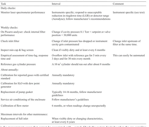
The gas sampling system consists of several parts each requiring its own maintenance scheme. Maintenance of each separate item is particularly important since mal-function of either can lead to erroneous measurements. Maintenance of each sub-system is described in the follow-ing sections and the timfollow-ing is compiled in Table 5.

Pump

Vacuum pumps run constantly in order to maintain low pressure in the measurement cell. When using scroll pumps

under continuous usage, the Teflon gaskets inside the pump

wear out following the manufacturers working hours. While some pumps have working hour counters, others do not. If such counter is not available, it is recommended to replace the gaskets every 14-16 months. This can either be done manually using a servicing kit or by sending the pump to the manufacturer. Following replacement of the gasket,

it must be confirmed that the pump returned to similar per -formance as before. Regular changes of the gaskets avoid

a contamination of the cell with Teflon particles following

pump failure, which is a common scenario. Alternative a lengthy tube between analyser and pump also avoids

back-flushing of debris.

Screw pumps do not require seals and this particular maintenance, but long-term experience is limited.

Flow and pressure meter

Flow meters should be checked for correct performance on a regular time schedule (every 6 months) against a

in the measurement occur that cannot be associated with changes in inlet characteristics. Continuous operation of

the flow controller is crucial to monitor filter, tube perfor

-mance and flow rate of the gas under observation.

Tube

There is no recorded evidence that tube

contamina-tion is a major issue for measuring fluxes of CH4 and N2O.

The less the H2O fluctuates as it reaches the analyser, the

smaller its effect on the CH4 and N2O measurement. Thus,

the flux attenuation for H2O caused by increased

adsorp-tion/desorption reduces the magnitude of the GHG flux

correction due to water vapour effects and is in principle helpful. Clearly, contamination to a degree that it can affect the instrument mirrors need to be avoided. Thus, it is re- commended to renew the main inlet line at least every six years, but also when visibly dirty or when any of the qua- lity checks indicate a change in performance. Reference

gas measurements, flow rate measurements must be per -formed before and after the tube has been exchanged and

noted. Check the system for leaks when the gas sampling

set up is exchanged or modified by overflowing the system

with zero air at the inlet.

By contrast, the inlet section upstream of the first filter should be replaced with each filter change.

Filter

The conditions apply as for the infrared gas

ana-lyser (IRGA) for measuring CO2 and H2O. The installed

Swagelok FW-2 µm pore diameter filter and additional ele -ments can be cleaned numerous times. The recommended cleaning procedure is as follows:

• Use clean filtered compressed air (zero-grade air or

ultra-pure nitrogen) to blow out the large particulate matter, around 300 kPa of over-pressure, in the reverse

flow direction.

• Place the filter in a sonic bath filled with chemistry

grade glassware cleaner. Leave in the bath for about two hours.

Table 5. Calibration and maintenance schedule for closed-path sensor setups

Task Interval Comment

Daily checks:

Monitor laser spectrometer performance Instruments specific; respond to unacceptable reduction in ringdown time (LGR) or detector range (Aerodyne); follow manufacturer’s recommendations

Instrument specific (see text)

Weekly checks:

On Picarro analyser: check internal filter

performance Change if cavity pressure 0.1 Torr < setpoint or valve position < 30,000 units

Check inlet filter Change if inlet pressure has dropped or instrument

cavity gets contaminated Change inlet upstream of filter at the same time. Inspect rain cap & bug screen Clean if visibly dirty and at least every 6 months

Empirical assessment of time-lag, response

time and Overflow inlet with reference gas for 5 min every 3 days and for 30 min every month This can easily be automated Reference gas cylinder pressure A 10 m3 _{cylinder should run out after about 8 months}

About annually:

Calibration for reported gases with certified

standard Annually mandatory

Calibration for H2O with dew point

generator Annually mandatory

Replacement of pump gasket Typically 14-16 months, follow manufacturer guidelines

Service air conditioning of the enclosure Follow manufacturer’s guidelines

Calibration of flow meter 6 months, or when readings change unexpectedly

Maximum intervals for other maintenance:

• Flush the filter with distilled water, first in the reverse flow direction and then in the flow direction.

• Use clean compressed air to blow out the large

par-ticulate matter, about 200 kPa, first in the reverse flow

direction and then in the forward direction.

• Rinse again in the sonic bath filled with clean distilled water for one hour and then use clean filtered com

-pressed air to blow out the clean filter, about 300 kPa, first in the reverse flow direction and then in the direc

-tion of flow. Allow the filter to dry for 24 h in a clean

and dry location.

• Visually inspect the retainer screens on both sides of

the filters inlet/outlet for corrosion. If corrosion/rust appears on the retainer screens, discard the filter. • The filter should also be discarded if there is evidence

that it is compromised (e.g. visible contamination of inlet line or degradation of measurement cell characteristics).

For the Picarro analysers, regular maintenance of the

additional instrument-internal inlet filters should be per

-formed to ensure adequate flow rates through the system.

Filter cleaning becomes necessary when the Cavity pres-sure drops below 0.1 Torr of the setpoint value and the Inlet

Valve Position drops significantly below 30 000 digital

units.

Rain cap and bug screen

Both rain cap and bug screen need to be cleaned regu-larly to minimise the potential for dirt to enter the sampling

tubes and avoid reductions in pressure and flow rate in the

sampling tube.

Temperature controlled housing

The air conditioning of the enclosure or cabin needs to be kept in good working conditions following the manufac-turer’s advice. The temperature sensor that monitors and records the housing temperature needs to be kept in good working order.

Monitoring of the laser absorption spectrometer performance

In order to operate a laser absorption spectrometer reli-ably, continuous monitoring of a few internal variables is essential. These include the mirror cleanliness, which can either be done via monitoring of the cavity ringdown time (e.g. LGR), the average detector range (e.g. Aerodyne) or the “baseline loss of the cavity” (Picarro), which is the inverse of the product of ringdown time and the speed of light. The cell pressure also needs to be monitored closely and action taken if it drifts. An overall monitoring of the instruments performance according to manufacturer’s re- commendations is recommended.

Validation measurements / calibration

Besides regular monitoring of the system performance and gas sampling sub-units, annual validation

measure-ments of a specific reference gas and a zero reference are

mandatory, together with calibration of the H2O

measure-ment using a dew point generator. The way calibrations need to be applied to the data differs between manufac-turers. The Picarro analysers apply a linear calibration internally which can be changed by the user, by updating a span and intercept value. Similarly, the Los Gatos

Research instruments, with a performance specification of

less than +/- 1% total uncertainty, allow the user the option to apply a 1-point calibration which will modify the internal (factory) calibration. The Aerodyne instruments report the

concentration that is derived from first principles and do not

apply any further calibration to the reported data, although the typical absolute values for N2O and CH4 concentration

are within 2% of the actual values in the Aerodyne instru-ments, approaching the accuracy of the standards available. The water absolute values are typically within 3% of abso-lute values. Dealing with all these variations of the various analysers requires the continuous submission of a span and offset correction to the ICOS Ecosystem Thematic Centre (ETC), which need to be applied in post-processing, based on the calibration results. If the internal calibration of the LGR and Picarro instruments is adjusted, the span and off-set would be 1 and 0, respectively.

Span validation measurements should be performed

with a known reference gas (e.g. pressurized gas) at two

concentrations (one near ambient and one higher). Thereby the pressurized gases have to be calibrated against a

high-precision standard (e.g. WMO, NIST, WGAA etc.). The

goal is to maintain working span gases that have 1% accu-racy, or better, and are traceable to a known international

standard. The high precision calibration gas certificate

needs to be provided to the ETC and so do the results of the annual reference measurements.

A two-point calibration with a zero is not generally advised because absorption spectrometers are not normally

optimised to detect zero concentration, and the spectral fit

can be lost when no absorption peak is found. Where pos-sible, however, the calibration of the zero can be checked with a zero gas which may be synthetic air minus the trace

gas of interest, or pure N2. Another approach to receive

a zero measurement can be achieved by pumping down the pressure in the sampling cell to measure “nothing” (e.g. Aerodyne).

Calibrations should be performed for all gases reported by the instrument that are submitted to the ICOS database or used in corrections (e.g. H2O). Special care needs to be

taken with calibrations of CO2 based on measurements of

the 13_CO

2 isotopologue; the isoptopic abundance of the

standard, which may differ greatly from ambient air, needs

to be known and taken into account (Brown et al., 2017;

Tans et al., 2017).

For the H2O calibration, dewpoint generators gene-

rally control their own flow and cannot cope with pres -sure changes on the outlet. Thus, the gas analyser needs

to sub-sample from the dewpoint generator outlet flow via

Based on the annual calibration, measurement drifts in the laser absorption spectrometer can be detected and cor-rected for. Internal instrument offsets may not be as critical

for high-frequency flux measurements, but are problematic

and are commonly corrected for internally (e.g. Aerodyne

Research Inc.). In addition to the annual calibration, the instrument performance needs to be assessed regularly with

the reference gas overflow inlet solenoid valve as detailed

above (for 5 min every 3 days; for 30 min, once a month). Quantification of storage flux

So far, there is little evidence that the problem of the

storage flux quantification for CH4 and N2O differs

funda-mentally from that for CO2.

Storage measurements for non-CO2 gases are manda-

tory for stations that measure these gases and where the EC system is placed at a height of 4 m or above. They can be either mandatory or only recommended for tower heights between 2 and 4 m, depending on the relevance

of fluxes (tested by estimating the difference between sto-rage fluxes calculated with a single point at the EC level and those calculated with a concentration profile; for de-tails see the ICOS protocol on storage term

quantifica-tion of this issue). In addiquantifica-tion to specifying the minimum number of sampling points according to the EC measure-ment height and their displacemeasure-ment, ICOS allows for three

possible set-ups to sample the concentration profiles.

In the ‘separate’ scheme (named ‘A’ in the protocol), concentrations at each inlet (height) are continuously sam-pled by a dedicated gas analyser. In the ‘sequential’ scheme (‘B’ in the protocol) a single gas analyser is used to

meas-ure the full profile system by the continuous and sequential

sampling of each level. Gas concentrations from each inlet

are averaged into ad-hoc mixing volumes before being

measured. Measurements can be performed for a few minu- tes across the beginning and the end of the EC averaging period. The ‘simultaneous’ scheme (‘C’ in the protocol) deploys one single gas analyser to continuously measure air from all the inlets after having been mixed together.

Air from individual sampling lines flows into a single

mixing volume causing a spatial integration of

concen-trations. The volume (flow rate) of air sampled from any

given height needs to be proportional to the vertical extent

of that given layer. Details and technical specification of

each sampling scheme are provided in the ICOS protocol

on storage term quantification of this issue and the ICOS

Ecosystem Instructions. The high cost associated with

analysers for CH4 and in particular N2O makes Scheme

A rather unattractive. Scheme B and C are both potential options. The requirement for the analysers used to quan-tify storage is similar to that of the EC analysers and this in particular also relates to need for an internal H2O mea-

surement. However, a response time of 10 s is sufficient,

together with 10 s detection limits of 1 ppb. Because an increasingly larger number of analysers can meet these

requirements, this paper does not attempt to provide a com- plete overview. Some photo-acoustic analyser (e.g. INNOVA Air Tech Instruments, Ballerup, DK) are known to have

significant cross-interferences between compounds and these are difficult to eliminate completely (Neftel et al., 2006) . Such instruments must be avoided to guarantee the most accurate measurement under all conditions.

In case the sequential sampling scheme is used, one of

the inlets of the vertical profile should be placed at the EC

system height so that potential sampling biases between the gradient and EC analysers can be corrected for.

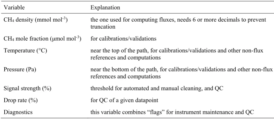
Data acquisition

The compulsory output variables are described here for closed-path and in Appendix 1 for open-path analysers. The standard acquisition frequency is 10 Hz for EC concentra-tion data and 1 Hz for other data. For closed-path analysers, the data that should be recorded at EC data frequency include the CH4 dry mole fraction (in nmol mol-1) and/or

the N2O dry mole fraction (nmol mol-1) as well as the H2O

mole fraction (mmol mol-1_{), together with cell temperature}

(°C) and cell pressure (Torr).

In addition, a data flag should be included that should

differentiate between (i) valid EC data, (ii) valid gradient data, (iii) valid calibration data and (iv) invalid data (e.g.

servicing, sensor obstruction). For the recording, the digital data stream from the analysers should be used and a high-accuracy time-stamp should be included that indicates when the measurements were taken. This time-stamp should be consistent with the one used for the recording of the sonic anemometer data to allow precise merging of the datasets during post-processing. If different data acquisition sys-tems are used, these need to stay on the same time-stamp,

e.g. using a precision timing protocol (IEEE, 2008). The

state of the solenoid valve that forms part of the reference

gas overflow inlet needs to be recorded as another flag. The inlet flow (l min-1_{) and pressure [kPa] should be}

recorded at a frequency of at least 1 Hz. All relevant diag-nostic analyser variables should be recorded and submitted to the ETC, but this can be recorded at a lower frequency and will depend on the instrument. The LGR analysers report various system health parameters and all measured variables that affect the measured gas concentration, as well as the the ringdown time (ms), which is an indicator

of mirror reflectivity. If a significant change occurs in this

ringdown time (for example, greater than 20% reduction), the precision of the instrument may be reduced.

The Aerodyne QCL instruments save diagnostics into

a different (*.stc) file than the concentrations (*.str) and

this includes important control indicators such as the range (the light level detected by the detector), internal valve states, laser temperature and voltage, as well as

informa-tion on the spectral fit. The number of diagnostics that can

be saved on Picarro analysers appears to have increased as