Slope Optimal Designs for Third Degree Kronecker Model Mixture Experiments

(1)

http://www.sciencepublishinggroup.com/j/ajtas doi: 10.11648/j.ajtas.20170604.11

ISSN: 2326-8999 (Print); ISSN: 2326-9006 (Online)

Slope Optimal Designs for Third Degree Kronecker Model

Mixture Experiments

Cheruiyot Kipkoech

1

, Koske Joseph

2

, Mutiso John

2

1_{Department of Mathematics and Physical Sciences, Maasai Mara University, Narok, Kenya} 2

Department of Statistics and Computer Science, Moi University, Eldoret, Kenya

Email address:

[email protected] (C. Kipkoech)

To cite this article:

Cheruiyot Kipkoech, Koske Joseph, Mutiso John. Slope Optimal Designs for Third Degree Kronecker Model Mixture Experiments. American Journal of Theoretical and Applied Statistics. Vol. 6, No. 4, 2017, pp. 170-175. doi: 10.11648/j.ajtas.20170604.11 Received: October 13, 2016; Accepted: October 28, 2016; Published: June 1, 2017

Abstract:

Mixture experiments are special type of response surface designs where the factors under study are proportions of the ingredients of a mixture. In response surface designs the main interest of the experimenter may not always be in the response at individual locations, but the differences between the responses at various locations is of great interest. Most of the studies on estimation of slope (rate of change) have concentrated in Central Composite Designs (CCD) yet mixture experiments are intended to show the response for all possible formulations of the mixture and to identify optimal proportions for each of the ingredients at different locations. Slope optimal mixture designs for third degree Kronecker model were studied in order to obtained optimal formulations for all possible ingredients in simplex centroid. Weighted Simplex Centroid Designs (WSCD) and Uniformly Weighted Simplex Centroid Designs (UWSCD) mixture experiments were obtained in order to identify optimal proportions for each of the ingredients formulation. Derivatives of the Kronecker model mixture experiment were used to obtain Slope Information Matrices (SIM) for four ingredients. Maximal parameters of interest for third degree Kronecker model were considered. D-, E-, A-, and T- optimal criteria and their efficiencies for both WSCD and UWSCD third degree Kronecker model were obtained. UWSCD was found to be more efficient than WSCD for almost all the points in the simplex designs, therefore recommended for more optimal results in mixture experiments.

Keywords:

Kronecker Model, Optimal Designs, Slope Information Matrices (SIM), Weighted Simplex Centroid Designs, A-, D-, E- and T-Optimality

1. Introduction

Response surface methodology (RSM) is a collection of mathematical and statistical tools or techniques that are useful for modeling and analysis of problems in which a response of interest is influence by several ingredients and the objective is to optimize this response, Montgomery (2001). Response Surface Methodology is an important subject in the statistical design and analysis of experiments. Mixture experiments are special type of RSM associated with the investigation of the m factors, assumed to influence the response only through proportions in which they are blended together. The mixture ingredients t1, t2,…, tm are such that

ti≥0 and further restricted by

∑

ti =1. Thus the experimental

domain is the probability simplex

1

( ,..., , ) [0,1] : 1

m m

m m i

i

T t t t t

=

 

′

= = ∈ = 



∑

 (1)

Under experimental condition t∈T_m, the response Y_t is taken to be a real-valued random variable. In a polynomial regression model the expected value E Y( )t is a polynomial

(2)

mean response. From the work of Hader and Park (1978), Huda and Al-Siha (1999) and Huda (2006), it is clear that most of the work has been done on central composite designs hence there was a need to extend the concept of slope to mixture experiments third degree Kronecker, this method was therefore used for proper identification of the ingredients ratio that leads to an optimal response.

The S-polynomial is given as,

1 , 1

( ) ( )

m m m

t i i ij i j ijk i j k i i j i j k

i j

E Y f t θ θt θ t t θ t t t

= = < < <

′

= =

∑

+

∑

+

∑∑ ∑

₍₂₎

and the homogeneous third-degree K-polynomial is

1 1 1

( ) ( ) ( )

m m m

t ijk i j k

i j k

E Y f t θ t t t θ θ t t t

= = =

′ ′

= = ⊗ ⊗ =

∑∑∑

(3)

in which the Kronecker powers t⊗3 = ⊗ ⊗(t t t), (m +1)3

vectors, consists of pure cubic and three-way interactions of components of t in lexicographic order of the subscripts and with evident that third-degree restrictions are

ijk ikl jik jki kij kji

θ =θ =θ =θ =θ =θ for all i j, and k

All observations taken in an experiment are assumed to be of equal unknown variance and uncorrelated. The moment

matrix

1

( ) ( ) ( ) ( ) ( )

t

t t

j j j j

M w t f t f t f t d

η

η η

=

∑

=

∫

for the third

degree Kronecker model has all entries homogeneous in

degree six and reflects the statistical properties of a designη. The moment matrix can be partition into sub moments according to the number of ingredients in a simplex centroid design as follows

1 1 2 2

( ) ( ) ( ) +...+ m ( m)

M η =αM η +α M n α M n (4) For Uniformly Weighted Simplex Centroid Designs (UWSCD), the weights are assumed to be distributed uniformly in the sub moments matrices. Hence

1 1 2 ... m=m

α α

= = =

α

and their moment matrix is given as,

1 1 1

1 2

( ) m ( ) m ( ) +...+m ( m)

M

η

= M

η

+ M n M n (5)

2. Information Matrix

Consider the Euclidean unit vectors in ℜm denoted by

1, 2,..., m

e e e and the set for

, e for i<j<k, i,j,k={1,2,...,m}

ii j i i j ijk i j k

e = ⊗ ⊗e e e = ⊗ ⊗e e e ₍₆₎

Let K be a k×scoefficient matrix such that

( ) 3 ₁ 1 2 3

( ; ; ) m m

K = K K K ∈ℜ × + (7)

where

' 1 ' 1

1 2 3( 1) 3 ( 1)( 2)

1 , 1 , , 1

, [ ( ) ] and ( )

m m m

iii i m iij iji jii i m m m ijk

i i j i j k

i j i j k

K e e K ₋ e e e e K ₋ ₋ e

= = =

< ≠ ≠

=

∑

=

∑

+ + =

∑

The Kronecker model of the full parameter vector θ_∈ℜm3

is not estimable. When fitting this model, the parameter subsystem considered in this study can be written as

( ) 3

1

1 1

3( 1) , 1

1 ( 1)( 2)

, , 1

( )

' ( ) for all

( )

iii i m m

m m

iij iji jii m

i j m

ijk m m m

i j k i j k

K

θ

θ θ θ θ θ

θ

≤ ≤

+ −

=

− − = ≠ ≠

 

 

 

  

=  + + ∈ℜ ∈ℜ

 

 

 

 

∑

(8)

where m3 (m1)

K∈ℜ × +

The parameter subsystem K′θ of interest is a maximal parameter system in the full parameter model. The information matrix for the parameter subsystem is given by

( ( )) ( ) ` ( )

k

C M η =LM η L∈NND s (9)

where L is the left inverse of coefficient matrix K and is

defined by

1

` ( ` ) `

L= K K − K (10)

Thus the information matrices for K`θ are linear transformation of moment matrices.

3. Application in Four Factors Mixture

Experiments

Using simplex restrictions, we obtained the optimal weights for WSCD,

1, 2, 3 and 4

α α α

α

as 4/15, 6/15, 4/15 and

1/15 respectively. From equation (4), we have the moment matrix for four factors mixture experiments as,

6

4 4 1

1 2 3 4

15 15 15 15

( ) ( ) ( ) ( ) ( )

M

η

= M

η

+ M n + M n + M n (11)

where,

1

1 4 111 111 222 222 333 333 444 444

( ) [ ( ) ' ( ) ' ( ) ' ( ) ']

M η = e e +e e +e e +e e (12)

1

2 384 1 1 1 1 1 1 2 2 2 2 2 2

3 3 3 3 3 3 4 4 4 4 4 4

5 5 5 5 5 5 6 6 6 6 6 6

( ) [( )( ) ' ( )( ) '

( )( ) ' ( )( ) ' ( )( ) ' ( )( ) ']

M d d d d d d d d d d d d

d d d d d d d d d d d d d d d d d d d d d d d d

η = ⊗ ⊗ ⊗ ⊗ + ⊗ ⊗ ⊗ ⊗

+ ⊗ ⊗ ⊗ ⊗ + ⊗ ⊗ ⊗ ⊗

(3)

1 2916

3 1 1 1 1 1 1 2 2 2 2 2 2

3 3 3 3 3 3 4 4 4 4 4 4

( ) [( )( ) ' ( )( ) '

( )( ) ' ( )( ) ']

M f f f f f f f f f f f f

f f f f f f f f f f f f

η = ⊗ ⊗ ⊗ ⊗ + ⊗ ⊗ ⊗ ⊗

+ ⊗ ⊗ ⊗ ⊗ + ⊗ ⊗ ⊗ ⊗ (14)

1 4 4096 64

( )

M

η

= J (15)

also,

1 4 4 3 2 4 2 4 3 4 1 4 4 4 1 3

4 4 1 3 5 4 1 2 6 4 2 3

(1 ), (1 ), (1 ), (1 ),

(1 ), (1 ) , (1 )

d e e d e e d e e d e e d e e d e e d e e

= − − = − − = − − = − −

= − − = − − = − −

1 (14 4), 2 (14 2), 3 (14 3), 4 (14 1),

f = −e f = −e f = −e f = −e

1

1 0 0 0

e      

=_{ }

   

, 2

0 1 0 0

e      

=_{ }

   

, 3

0 0 1 0

e      

=_{ }

   

and 4

0 0 0 1

e      

=_{ }

   

The Uniformly Weighted Simplex Centriod Designs (UWSCD) for four ingredients were assumed to assign uniform weights to the four elementary centroid designs,

1, , and 2 3 4

n n n n , such that all weights are equal. That is,

1= 2 3 4 0.25

α α =α =α = (16)

The moment matrix for uniformly weighted simplex centriod designs in (5) for four ingredients is given by

1 2 3 3

( ) 0.25 ( ) 0.25 ( ) 0.25 ( ) 0.25 ( )

M η = M η + M n + M n + M n (17)

where,

1

( )

M η , M n( 2), M n( )3 and M n( 4) are given in (12),

(13), (14) and (15) respectively.

The coefficient matrix K for the four ingredients parameter subsystems of interest in (7) and (8) is given as

(

K ,1 2, 3

)

K= K K (18)

where

4

1 111 1 222 2 333 3 444 4

1

' ' ' ' '

iii i i

K

e

e e e e e e e e e

=

∑

= + + + +

{

}

3 1 2 9

1

112 121 211 1 122 212 221 2 133 313 331 3 144 414 441 4 9

) '

( ) ' ( ) ' ( ) ' ( ) '

(

iij iji jii i

ij i j

K e

e e e e e e e e e e e e

e

= ≠

 

 

=  + + 

 

 

= + + + + + + + + + + +

∑

and

4 1 3 24

1

123 132 231 213 312 321 124 134 142 143 214 234 24

241 243 314 324 341 342 412 413 421 423 431 432

(

)

ijk ijk i j k K

e e e e e e e e e e

e e e e e e e e e e e e

e

= ≠ ≠

   

=  

   

= + + + + + + + + + + +

+ + + + + + + + + + + +

∑

The left inverse L in (10) for four ingredients is given as,

(

1 2 3

)

' K , 6 , 24

L = K K (19)

4. Slope Designs

In response surface designs the main interest of the experimenter may not always be in the response at individual locations but, the differences between the responses at various locations may be of greater interest, Herzberg (1967),

Box and Draper (1980), Huda and Mukerjee (1984) and Huda (2006).

We know that to maximize the response, the movement of the design center must be in the direction of the directional

derivatives of the response function, that is, Yt

t

∂

∂ . Let H be a

(4)

1 2

'( ) '( ) '( ) , , ...,

m

f t f t f t H

t t t

′

_∂ _∂ _∂ 

= 

∂ ∂ ∂

  (20)

Therefore,

(

)

( )

(

)

( )

(

)

( )

(

)

( )

(

)

( )

(

)

( )

1 1 1

3 3 3

1 1

3 3

1 1

3 3

1 1

3 3

2 2 2 2 2 1

3₁ 0 0 0 ₃ _{1 2} _{1 3} _{1 4} ₂ ₃ ₄ ₄ _{2 3} _{2 4} _{3 4}

2 1 2 2 2 2 1

0 3₂ 0 0 ₃ ₁ ₃ _{1 2} _{2 3} _{2 4} ₃ ₄ ₄ _{1 3} _{1 4} _{3 4}

2 1 2 2 2 2 1

0 0 3₃ 0 ₃ ₁ ₂ ₃ _{1 3} _{2 3} _{3 4} ₄ ₄ _{1 2} _{1 4} _{2 4}

2 1 2 2 2 2

0 0 0 3₄ ₃ ₁ ₂ ₃ ₃ _{1 4} _{2 4} ₃

H

t t t t t t t t t t t t t t t t

t t t t t t t t t t t t t t t t

t t t t t t t t t t t t t t t t

t t t t t t t t t

=

+ + + +

+ +

(

) (

1

)

4 4 1 2 1 3 2 3

t t t +t t +t t

 

 

 

(21)

Using (11) and (19), we obtained the information matrix for Weighted Simplex Centroid Designs (WSCD) as

11 12 13

2 12 22 23

13 23 33

' '

c c c

C c c c

c c c

 

 

=_ _

 

 

(22)

where,

4 4

11 11 4 11 4 11 11

4 4

12 12 4 11 4 12 12

4 4

22 22 4 22 4 22 22

; 688.4 10 , 12.40842 10

; 67.98697 10 , 43.68878 10

; 220.42181 10 , 172.77722 10

c x I y J x y

− −

= + = × = ×

4 13 13 4 13

4 23 23 4 23

4 33 22 22

1 ; 20.36716 10

; 133.92168 10

; 225.43724 10

c x x

c x I x

c x x

−

= = ×

The derivative matrix (21) together with information matrix (22) were used to obtain Slope Information Matrices (SIM) at different points of the simplex. At (1, 0, 0, 0), the slope information matrix is given as,

4 4

3

41 4 4

3 3

6307.40393 10 111.67574 10 (1 ') 111.67574 10 (1 ) 43.6887 10 SIM

J

− −

 _× _× 

=_ _

× ×

  (23)

At the binary blend point (0.5, 0.5, 0, 0) the slope information matrix is of the form

4 4 4

2 2 2

42 4 4

2 2

399.23626 10 ( ) 48.7828 10 25.5644 10

25.5644 10 13.14636 10

I J J

SIM

J J

− − −

− −

 _× ₊ _× _× 

= 

× ×

  (24)

At the point (0.333, 0.333, 0.333, 0) the slope information matrix is

4 4 4

3 3 3

43 4 4

3

84.2478 10 ( ) 22.98775 10 12.51869 10 (1 )

12.51869 10 (1' ) 7.0857 10

I J

SIM

− − −

− −

 _× ₊ _× _× 

=_ _

× ×

  (25) At the point (¼, ¼, ¼, ¼), the slope information matrix is given as

44

549/125029 61156/30546869 4185/2854654 4185/2854654 61156/30546869 3764/639087 5241/2207668 61156/30546869 4185/2854654 5241/2207668 549/125029

SIM =

4185/2854654 4185/2854654 61156/30546869 4185/2854654 549/125029

 

 

 

(26)

Using (17) and (19), we obtained the information matrix for uniform weighted simplex centroid designs as,

11 12 13

2 21 22 23

13 23 33

' '

u

c c c C c c c c c c

 

 

= 

 

 

(5)

where c11, c12, c13, c22, c23 and c33are given as

4 4

11 11 4 11 4 11 11

4 4

12 21 12 4 11 4 12 12

4 4

22 22 4 22 4 22 22

; 638.8782 10 , 8.8354 10

' ; 44.2062 10 , 35.3124 10

; 148.05 10 , 169.7616 10

c x I y J x y

c c x I y J x y

c x I y J x y

− −

= + = × = ×

= = + = × = ×

= + = × = ×

4 13 31 13 4 13

4 23 32 23 4 23

4 33 22 22

' 1 ; 30.0810 10

' 1 ; 224.4348 10

; 475.0416 10

c c x x

c x x

−

= = = ×

= = ×

The derivative matrix (21) together with information matrix (27) were used to obtain Slope Information Matrices (SIM) at different points of the UWSCD. At point (1, 0, 0, 0), the slope information matrix is given by,

4 4

3

41 4 4

3 3

5829.4224 10 79.5186 10 (1' )

79.5186 10 (1 ) 35.3124 10

u SIM

J

− −

 _× _× 

=_ _

× ×

  (28) For binary blends at points (½, ½, 0, 0), we have information matrix as,

4 4 4

2 2 2

42 4 4

2 2

365.92289 10 38.46044 10 22.25155 10

22.25155 10 ' 13.30321 10

u

I J J

SIM

J J

− − −

− −

 _× ₊ _× _× 

= 

× ×

  (29) We obtained slope information matrix at the ternary point (0.333, 0.333, 0.333, 0) as,

4 4 4

3 3 3

43 4 4

3

76.08877 10 ( ) 21.21016 10 14.0479 10 (1 )

14.0479 10 (1' ) 10.16018 10

u

I J

SIM

− − −

− −

 _× ₊ _× _× 

=_ _

× ×

  (30) At the central point (¼, ¼, ¼, ¼) of the simplex centroid design, we have the slope information matrix given as,

44

0.004131819 0.002094689 0.001552438 0.001552438 0.002094689 0.005561169 0.002341674 0.002094689 0.001552438 0.002341674 0.004131819 0.001552438 0.001552438 0.002094689 0.0015

u

SIM =

52438 0.004131819

 

 

 

(31)

5. Optimal Values for Slope Information

Matrices (SIM)

Optimal designs are experimental designs that are generated based on a particular optimality criterion and are generally optimal only for a specific statistical model. The optimality properties of designs are determined by their moment matrices, Pukelsheim (1993). The amount of information inherent to Ck(M(η)) is provided by ϕp-criteria

with Ck(M(η))∈ PD(m), defined by:

1 min

1

( )

( ) det( ) 0

0,

s p

p p s

C if p C C if p

traceC if p

λ ϕ

 _{= −∞}

 

= =



  _{≠ ±∞}

 



(32)

We obtained the optimal values for both Weighted Simplx Centroid (WSC) designs and Uniform Weighted Simplex Centroid Designs (UWSCD) for four ingredients mixture experiments.

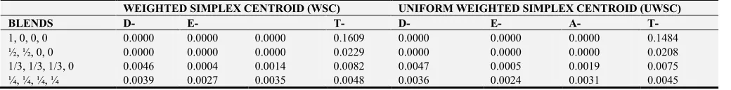
Table 1. _{Optimal Values for Four Ingredients.}

WEIGHTED SIMPLEX CENTROID (WSC) UNIFORM WEIGHTED SIMPLEX CENTROID (UWSC)

BLENDS D- E- T- D- E- A- T-

1, 0, 0, 0 0.0000 0.0000 0.0000 0.1609 0.0000 0.0000 0.0000 0.1484 ½, ½, 0, 0 0.0000 0.0000 0.0000 0.0229 0.0000 0.0000 0.0000 0.0208 1/3, 1/3, 1/3, 0 0.0046 0.0004 0.0014 0.0082 0.0047 0.0005 0.0019 0.0075 ¼, ¼, ¼, ¼ 0.0039 0.0027 0.0035 0.0048 0.0036 0.0024 0.0031 0.0045

Uniformly Weighted Simplex Centroids Design (UWSCD) was observed to yield more optimal values than Weighted

(6)

6. Efficiencies for Four Ingredients

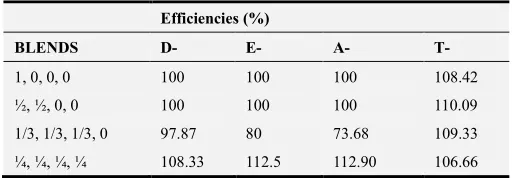
The efficiency of WSCD over UWSCD at different point of the simplex centroid designs were summarized as

Table 2. _{Efficiencies for Four Ingredients.}

Efficiencies (%)

BLENDS D- E- A- T-

1, 0, 0, 0 100 100 100 108.42

½, ½, 0, 0 100 100 100 110.09

1/3, 1/3, 1/3, 0 97.87 80 73.68 109.33

¼, ¼, ¼, ¼ 108.33 112.5 112.90 106.66

From Table 2, at (1, 0, 0, 0) and (½, ½, 0, 0), there was no difference between the two designs in their D-, E- and A- efficiency. However, UWSCD was 8.42% and 10.09% more T- efficient than WSCD at respective blends. For ternary mixture (0.333, 0.333, 0.333, 0), WSCD was 2.13%, 20% and 26.32% more D-, E- and A- efficient than UWSCD respectively. It was also observed that WSCD was 9.33% less T-efficient than UWSCD. At point (¼, ¼, ¼, ¼), UWSCD was 8.33%, 12.5%, 12.9% and 6.66% more D-, E-, A- and T- efficient respectively than WSCD. Generally, the D-, E-, A- and T-optimal values for Uniformly Weighted Simplex Centroid (UWSC) designs were better than those of Weighted Simplex Centroid (WSC) designs for four ingredients.

7. Conclusion

It was noted that Uniformly Weighted Simplex Centroid (UWSC) designs were more efficient than Weighted Simplex Centroid (WSC) designs. For more optimal results, the experimenter is advised to allocate weights in the mixture components uniformly. In UWSC design, the centroid point (¼, ¼, ¼, ¼) produced the most efficient results than any other point while WSC design yield the optimal results at point (0.333, 0.333, 0.333, 0) only.

References

[1] Box, G. E. P. and Draper, N. R. (1980). The variance functions of the diﬀerence between two estimated responses, J. Roy. Statist. Soc., B 42, 79-82.

[2] Draper, N. R. and Pukelsheim, F. (1998). Mixture models based on homogeneous polynomials. J. Statist. Plann. Inference 71 303–311.

[3] Hader, R. J. and Park, S. H. (1978). Slope-rotatable central composite designs, Technometrics, 20, 413-417.

[4] Herzberg, A. M. (1967). The behavior of the variance functions of the difference between two responses. J. Roy. Statist. Soc. B, 29, 174-179.

[5] Huda, S. (2006). Minimax designs for the difference between estimated responses for the quadratic model over hypercubic regions. Commun. Statist.- Theory meth.

[6] Huda, S. and Al-Shiha, A. A. (1999). On D-Optimal designs for estimating slope. The Indian Journal of Statistics. 61: B, 3, 488-495.

[7] Huda, S. and Mukerjee, R. (1984). Minimizing the maximum variance of the diﬀerence between two estimated responses, Biometrika, 71, 381-385.

[8] Kerich, G., Koske, J., Rutto, M., Korir, B., Ronoh, B., Kinyanjui, J. and Kungu, P. (2014). D-Optimal Designs for Third Degree Kronecker Model Mixture Experiments with An Application to Artificial Sweetener Experiment. IOSR Journal of Mathematics, 10 (6), 32-41.

[9] Korir, B. C. (2008),” Kiefer ordering of simplex designs for third-degree mixture models.” P. hd. Thesis Moi University. [10] Montgomery, M. D. (2001). Design and Analysis of

Experiments, 5th ed., John Wiley and Sons, New York. [11] Pukelsheim, F. (1993). Optimal design of experiments. Wiley,

New York.