On Nonnegative Integer-Valued Lévy Processes and Applications in Probabilistic Number Theory and Inventory Policies

2013; 2(5): 110-121

Published online August 30, 2013 (http://www.sciencepublishinggroup.com/j/ajtas) doi: 10.11648/j.ajtas.20130205.11

On nonnegative integer-valued Lévy processes and

applications in probabilistic number theory and inventory

policies

Huiming Zhang

*

, Jiao He, Hanlin Huang

Dept. of Mathematics and Statistics, Central China Normal University, Wuhan, China

Email address:

[email protected](Zhang H.)

To cite this article:

Huiming Zhang, Jiao He, Hanlin Huang. On Nonnegative Integer-Valued Lévy Processes and Applications in Probabilistic Number Theory and Inventory Policies. American Journal of Theoretical and Applied Statistics. Vol. 2, No. 5, 2013, pp. 110-121.

doi: 10.11648/j.ajtas.20130205.11

Abstract:

Discrete compound Poisson processes (namely nonnegative integer-valued Lévy processes) have the property

that more than one event occurs in a small enough time interval. These stochastic processes produce the discrete compound Poisson distributions. In this article, we introduce ten approaches to prove the probability mass function of discrete compound Poisson distributions, and we obtain seven approaches to prove the probability mass function of Poisson distributions. Finally, we discuss the connection between additive functions in probabilistic number theory and discrete compound Poisson distributions and give a numerical example. Stuttering Poisson distributions (a special case of discrete compound Poisson distributions) are applied to numerical solution of optimal (s, S) inventory policies by using continuous approximation method.

Keywords:

Probability Mass Function, Nonnegative Integer-Valued Lévy Processes, Probabilistic Number Theory,

Discrete Compound Poisson Distribution, (S, S) Inventory Policies

1. Introduction

Poisson distribution is a famous distribution in discrete distribution family, and it has important applications in social and economic sciences, physics, biology and other fields. For example, the number of passengers came to a bus stop, the number of particles emitted by radioactive substances, the number of microorganisms in a region under the microscope and so on. Poisson (1837) [25] tried to use the binomial distribution of several experiments to derive distribution function of the Poisson distribution in his representative work Recherches sur la probabilité des jugements en matière criminelle et en matière civile, précédées des règles générales du calcul des probabilités

2 3

(1 )

1 2 1 2 3 1 2 3

n

P e

n

ω

ω ω ω

ω −

= + + + + +

⋅ ⋅ ⋅ ⋯ ⋅ ⋅ ⋅ ⋅⋯

After about 100 years, de Finetti (1929) [6] initiated that the probability of an event in the interval [ ,t0 ∆ +t t0) of

Poisson Processes is λ∆ +t (o ∆t), (λ>0) and the probability more than one events iso(∆t). Khintchine [21] summarized the equivalent conditions of Poisson

distribution: zero initial conditions, stationary increments, independent increments, and orderliness (impossible of two or more events occurring in the same moment of time). In actual life, Poisson processes (distribution) is not an adequate model for the observed data that the possibility of two or more events occur at a given instant. Khintchine [21] also generalized the Poisson processes by giving more restrict of orderliness. As for a situation: during period of

t

, the number of cars that arrive at the terminal station can be regard to Poisson distribution, every car take

i

passengers with probability αi, thus the number of passengers who

arrive at the terminal station can not satisfy Poisson processes. So we assume that there are many events occurring in a small segment of length

t

. Hight [14] considered another situation: somebody might throw some letters (more than one) into a postbox at the same time.

2. Discrete Compound Poisson Model

2.1. Nonnegative Integer-Valued Lévy Processes

We employ the following definition due to [14].

Nonnegative integer-valued stochastic processes { ( )}X t t≥0

satisfy the following four conditions: (i) Initial condition:X(0)=0;

(ii) Stationary increments: the events occur in[ ,t t0 +t0)

only depends on

t

, and is not relevant to t0;

(iii) Independent increments: the events occur in

0 0

[ ,t t+t )is independent with the events which happen before t0;

(iv) Superimposition: the probability of

i

events

taking place between [ ,t t0 +t0) is:

1

( ), ( 1, 0, 0, )

( ) 1

i i i

i i

t t o t i

P λα λ α α

∞

=

∆ = ∆ + ∆ ≥ > ≥

∑

= .

Especially, when it applies to the inventory management theory, the number of consumers coming in a period of

t

can be seen to subject to the stuttering Poisson distribution (SPD). When the interval is small enough and the number has the property of geometric distribution, that is

(1 ) i, ( 1, 2, )

i

a = −α α i= ⋯ .

Galliher [12] applied SPD to the inventory management firstly, and named it as stuttering Poisson distribution. We will prove the explicit expression of probability mass function (pmf) of SPD in the following part. Definition 1

was put forward by Khintchine [21], where αi be

probability of nonnegative discrete distribution. Hight [14] still named stuttering Poisson distribution instead of discrete compound Poisson distribution existing in the broad sense of inventory management. There are some other names:

Pollaczek-Geiringer distribution, Generalized Poisson distribution, Composed Poisson distribution, Poisson power series distribution, Poisson par grappes distribution, Poisson-stopped sum distribution, Multiple Poisson distribution,

Infinite divisible distribution on the nonnegative integer. Readers can find more general information of Poisson distribution and discrete compound Poisson distribution in [18] and [14]. The wide range of applications with discrete compound Poisson, see [21], [16], [34], [12] and [2].

Definition 2. (Discrete compound Poisson distribution)

In particular, we say the discrete random variable X

satisfying the conditions above has a discrete compound Poisson (DCP) distribution with parameters

1 2 1

(α λ α λ, , ) R ( _i αi 1,αi 0,λ 0) ∞

∞

= =

∈

∑

≥ >

⋯ .

We denote it as

1 2

( , , )

X ∼CPα λ α λ⋯ .

If X ∼CP(α λ1 ,⋯,α λr ) ，we say X has a DCP

distribution of order r.

Remark 1. In the Section 3.8, we will show X t( ) have

compound Poisson sum properties.

Theorem 1. Discrete compound Poisson process X t( ) is a Markov chain with stationary independent increments. Let P ti( )=P{X t( )=i X(0)=0} . The pmf of DCP processes is

1 2

1 2 1

1 2 1 2 , N

( )

! ! !

( )

n

n n

i i i

k k k

k k k t n

n ik k

n

n

t e

k k P

k

t α α α λ λ

=

+ + + −

Σ = ∈

=

∑

⋯ ⋯

⋯ (1)

where N={0,1, 2,⋯}.

By the definition of Bell polynomial [4]:

1

1 0

( , , )

exp[ ]

! !

i i

i i i

i i

a B a a

x x

i i

∞ ∞

= = =

∑

∑

⋯ .

henceP ti( )satisfies

1

(1! , , ! ) ! ( ).

i i i

B α λt⋯i α λt =i P t

So P tn( ) can be expressed by Bell polynomial. The

indeterminate equation 1 , ( N)

n

i=iki n ki

Σ = ∈ is called

Diophant's equations. The depth theoretical properties and statistical applications of Bell polynomial with Diophant's

equations 1

n i=iki n

Σ = , see [30].

Theorem 2. If X t( )∼CP(α λ α λ1 t, 2 t,⋯) , then the

probability generating function (pgf) of X t( ) is

1 ( 1)

( ) , ( 1).

i i i

t s

P s eλ α s

∞

= −

∑

= ≤ (2)

Remark 2. We will give ten approaches to proof the pmf of DCP distribution and two to approaches proof the pgf of DCP distribution in Section 3.

Lévy processes { ( )}X t t≥0 satisfy the following four

conditions as follows: (i)P X{ (0)=0} 1, . .= a s ;

(ii)X t( )has independent increment; (iii)X t( )has stationary increment;

(iv) X t( ) is almost surely right continuous with left limits.

Lévy processes can derive Lévy–Khinchine formula (details can be seen in Bertoin(1996)). The characteristic

function ( )

E[ i X t ]

eθ of X t( )is

2 2

1 \{0}

1

exp ( 1 I ) ( )

2

i x

X R

aitθ σ θt t eθ i xθ _< w dx

 

− + − −

 



∫



,

wherea∈R,σ ≥0 , IA is an indicator function. And

( )

w dx is a measure which is called Lévy measure. It

satisfies

2

\{0}min{ ,1) ( )

R x w dx

∫ _{< ∞}.

compound Poisson process, and a pure jump martingale. By the definition of Lévy process, suppose

( ) x x

w dx =α λ δd , (3)

where δx is Dirac measures (or point measure) with

( ), ( N)

x

fdδ f x x

∫ _{= ∈} and 2

\{0}min{ ,1) ( )

R x w dx

∫ _{< ∞}. Because X t( ) is a integer value as well as the definition of w dx( ), we have

2 2

1 \{0}

1

( I ) ( ) 0

2 R X

aitθ− σ θt =t

∫

i xθ _< w dx =

.

Hence, the characteristic function of X t( )is

( )

1

E[ i X t ] exp[ ( ji 1)]

j j

eθ λt α e θ

∞

=

=

∑

− ,

Theorem 2 shows that the Lévy measure (3) we defined before is reasonable.

Discrete compound Poisson process is a continuous-time non-negative integer value Lévy process. Barndorff [2] put forward the integer-valued Lévy process, and he use it in latency financial econometrics.

2.2. Special Case

2.2.1. Hermite Distribution

When r=2 in definition 2, it called Hermite

distribution. The pmf is

[ ] ₂ 2

1 2

0

( ) ( 2 )! ! ( )

n

n i i n i

i

t n

P t t

n i i e

λ

α α λ− − =

−

− =

∑

.

The pmf above is gotten by the pgf of Hermite distribution expanded in terms of Hermite polynomial. More details can be seen in Kemp [19].

2.1.2. Stuttering Poisson Distribution

In inventory system, Galliher [12] use the DCP distribution with parameter X t( )∼CP(α λ α λ1 t, 2 t,⋯) to

describe the demands

,

where 1

(1 )

n

n

α λ_{= −}α α λ−

_.

_He

called it stuttering Poisson distribution.

The following parts show that the pmf of SPD can be expressed by Laguerre polynomial. We need a lemma. The power series solution of second-order linear differential equation

(1 ) 0

xy′′+ −x y′+ny=

is ( ) ( )

!

x n n x

n n e d x e

y L x

n dx

−

= ≜ , which is called Laguerre

polynomial.

We begin by proving a property of Laguerre polynomial. First, we need Lemma 1. It is the connection between Laguerre polynomial and pgf of SPD.

Lemma 1: The Taylor’s formula with respect to

t

of

1

1 ( , )

1

xt t

P t x e t

− −

=

− is 0 ( )

n n

n L x t

∞ =

∑

in t ≤ <r 1.

Proof: It is easy to prove that ( )

!

x n n x

n

e d x e

n dx

−

⋅ satisfies

ODE: xy′′+ −(1 x y) ′+ny=0 . Suppose

t

is a complex variable and assume that P t x( , )= −(1 t)−1e− −(1 t)−1xt is analytic in t ≤ <r 1 . Define the Taylor expansion of

( , )

P t x in t ≤ <r 1 is ₀ ( )n n

n a x t

∞ =

∑

. By the Cauchy

formula of higher order derivative of analytic function, the coefficient a xn( ) of power series is

1

1 ₁ 1

1 1 1

2 (1 ) 2 ( )

( )

!

x _{x n z}

x

n n

r r

z x n n x

n

e z e

e d dz

i i z x

e d x e

n dx

ξ ξ

ξ ξ

π ξ ξ π

− −

−

+ +

= − =

−

⋅ =

− −

= ⋅

∫

∫

Theorem 3：The pmf of SPD is

1

1 1

( ) n[ ( ) ( )] t

n n n

P t α L α λt L α λt e λ

α− − α− −

= − .

Proof: The pgf of SPD can be rewritten as follow by the Lemma 1 above:

1 1

1

(1 ) ( 1) ₁

0

1

0 0

( , )

1

( )( ) (1 )

1 1

= [ ( ) ( ) ]

i i

i

s t

t s t s

t n

n n

t n n

n n

n n

P s t e e e

e L t as as

e L t as L t as

α_λ α

α α λ λ α α

λ

λ

α λ α

α_λ α_λ

α α

∞ −

=

− _⋅

− − − −

∞ −

=

∞ ∞

− +

= =

∑

= =

−

= − −

− −

   

− − −

   

   

∑

∑

∑

( )

n

P t is the coefficient of n

s in the expanded formula of

( , ) P s t , hence

( )

0

1

( , ) 1 1

[ ( ) ( )] .

n t

n n

n

n n

s

L t L t

P s t

P t e

t

λ

α α

α λ λ

α α

=

− −

−

= − −

∂ =

∂

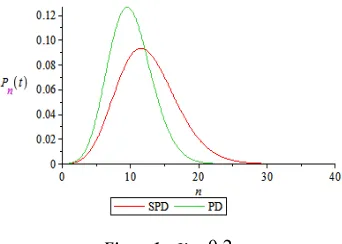
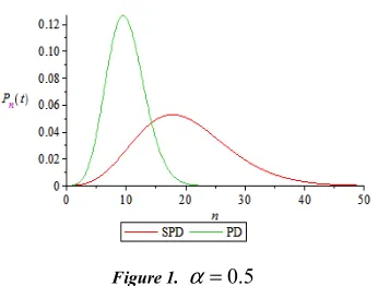
Letα =0.2 0.5,、 λt=10, plot the graphic in SPD and PD of y=P t_n( )by Maple 16.

Figure 1. α =0.5

The figure of SPD is more dwarfed than it is in PD from Fig.1 and Fig. 2 This is because the SPD have superimposed events occurred within a sufficiently small time interval, while the PD is not allowed. Number of incidents in a unit time is relatively more in SPD. More discrete compound Poisson distribution examples can be seen in Wimmer [32], it lists more than 100 special cases.

3. Ten Approaches to Prove the PMF of

Discrete Compound Poisson

Distribution

3.1. Lemma

Lemma 2. (Cauchy functional equation) Suppose f is

continuous on R , so f x( +y)= f x( )+ f y( ) for all

,

x y

∈

R

, Then f x( )=ax a( ∈R) . The proposition of Cauchy functional equation: Suppose f is continuous on

R , so f x( +y)= f x f y( ) ( ) for all

x y

,

∈

R

, Then

( ) ax( R)

f x =e a∈ .

Lemma 3. (Euler’s method of linear differential equation

with constant coefficients) Suppose a p-dimensional column

vector function x, P is an n-order coefficient matrix of

differential equation d dt =

x

Px.

Let F( )λ = −P λE , and detF( )λ =0 is the

characteristic equation of P. detF( )λ =0has different characteristic roots in the complex field. Suppose they are

1, 2, , m(m n)

λ λ ⋯ λ ≤ which have algebraic multiplicities

1, ,2 , m (1 2 m )

r r ⋯ r r + + + =r ⋯ r n . Then the particular solution of the equation is

1 1

1 [ ( ) ( )

2! 1

( ) ] , (1 ) ( 1)!

i i i

i i i

r r t

i i

i

t t

t e i m

r

λ

λ λ

λ

− −

= + + +

+ ≤ ≤

−

⋯

x E F F

F A

,

where the vector Ai satisfies equation i( ) 0

r i i λ =

F A .

Hence, the general solution of equation d

dt =

x

Px is

1 1 2 2 m m, ( ,1 2, , m are constants )

c c c c c c

= + + +⋯ ⋯

x x x x (4)

Lemma 4. (Polynomial of n-th power)

1 2

1 2 1

1 1

1 2 , N 1 2

( )

( !)

! ! !

n

n i

i n

i m m m i

i

k k k

l n

k k k m k n

k ik nk l

x x

m x

k k k

α α

α α α

∞

=

+ + = ∈

+ + + + =

= +

+ +

∑

∑

⋯

⋯ ⋯

⋯

⋯

⋯ ⋯

(5)

Another expression can be seen by Theorem 1 in [31]. In order to simplify the symbols, set the coefficient of l

x as

1 2

1 2 1

1 2

, N 1 2

! ! ! !

n

n i

i n

k k k

l n

m

k k k m k n

k ik nk l

N m

k k k α α α

+ + = ∈ + + + + =

=

∑

⋯ ⋯ ⋯

⋯ ⋯

.

Lemma 5. (Nilpotent matrix) I_n is a n -dimension

identity matrix, let shift matrix be 0

0 0

n

 

 

 

≜ I

N , if

1

i≥ +n , then i ₌0

N .

Lemma 6. (Faà di Bruno formula, [10]) If g and f

are functions with a sufficient number of derivatives, then we have

1 2 1 2

1 2

( ) , 0

2

)

1 1

(

! [

! !

( ) ( ) ( )

( ) ( ) ( ) ]

1 [ ( )]

( ( ))

! 2! !

n j

n

n

k k k i k n k k

n n

i n

nk n

n k k

i

k

n k k

f t d g f

f t f t

t

g f t t

n

d + + + = ≥

+ =

=

+ +

′ ′′ ⋅

=

∑

∑

⋯ ⋯

⋯

⋯

It is easy to verify Lemma 2 to Lemma 5, and the proofs can be found in many text books.

3.2. Univariate Multinomial Distribution Approximation

Now we discuss the generalization of n times of Bernoulli trials, and consider it under the situation: n→ ∞. This case is similar to univariate multinomial distribution (see [18]

p522): Suppose that there is a sequence of n independent

trials during segment length of t, where each trial has infinite

possible outcomes A A A0, 1, 2,⋯ that are mutually

exclusive and the probability of each outcomes can be written as :

0

0 1

( 1, 1) 1 ( ), i i ,

i i

o t

p λ t p α

∞ ∞

= =

= − ∆ + ∆

∑

=

∑

=

( ) i ( ),

i i

p = p A =λα∆ +t o ∆t

respectively. Let the occurrence of A ii( =1, 2,⋯)be deemed

to be equivalent to i successes and the occurrence of A0 be

deemed to be a failure. The number of successes X t( )

achieved in the n trials. When n→ +∞, the reader can see in Fig.3, we divide [ ,t t0 0+t) in to N pieces evenly, and

every interval is ∆t, that is lim

0 0 0 0 0 0

[ ,t t + ∆t),[t + ∆t t, + ∆2 t),⋯,[t +(N− ∆1) t t, + ∆N t). There is only one events choosing from A A A0, 1, 2,⋯ in

every[t0+ ∆h t t,0+ + ∆(h 1) t) (，h=1, 2⋯) . The number of

events A A1, 2,⋯ happened in all small intervals are limited,

while the number of A0 happened during [ ,t t0 0+t) is

infinite. To understand the process easier, we imagine there is a dice with infinite surfaces and each surface write one number0,1, 2,⋯. During time interval[ ,t t0 0+t) , after

t t

N =_∆ (approximate to an integer) times of tossing, figure out the probability that total number is n.

Figure 2. Divide t into infinity many interval of ∆tuniformly

When N→ +∞ , DCP distribution is equal to a

conditional multinomial distribution that was produced by a generalized infinite times independent repetition trial, the

pgf in one trial is

0

( ) i i, ( 1)

i

G s p s s

+∞

=

=

∑

≤ . Then

pgfP s( )=[ ( )]G s N of DCP can be written as:

0 2

0 1 0 1

0 1 0

, N 0 1

0

lim [ ( ! ) ]

! ! !

n

n u

n

k k k

N n n

N

k k k N k n

k k nk n

p p p

p N s

k k k

→∞ _{+ + = ∈}

⋅ + + + =

+ +

∑

+

⋯ ⋯

⋯

⋯ ⋯

⋯

by Lemma 5. According to the pgf, we know P tn( ) is the

coefficient of

s

n in the expansion formula of P s( ), since

0

1

, ( 1, 2, ), 1

i

i i

i

t t

p i p N t

N N α

λ

α λ ∞ _λ

=

= = ⋯ = − ， =

∑

where k1,…,kn are fixed nonnegative integers and the

constraint is n ₀

u= ku N

∑ ₌ . Then,

0 1 0 1

0 1

1

1

1 0 1

0 1

0 1 , N 0 1

0

( )

1

, N 1

0

1

!

! ! !

( )

lim [1 ]

( ) ( )

! !

( ) lim

lim

n

r u

n

n

n n

n u

n

k k k

n n

N

k k k N k n

k k nk n

N k k n

N

k k

k k N _{k k k N k}

n k k nk n

n

N

p p p

k k k

t N

k t

t k P

α λ α λ

α λ α λ

→∞ _{+ + = ∈}

⋅ + + + =

− + + →∞

+ +

+ + = ∈

⋅ + + =

→

+ ∞

+ + = −

=

⋅

∑

∑

⋯ ⋯

⋯

⋯ ⋯

⋯

⋯ ⋯

⋯

⋯ ⋯

1 1

1 1 2

1

2 , N 1

1

( 1) [ ( ) 1]

lim

( ) ( )

! !

n

n n

n u

n k k N

k k

k k t k k nk n k

n n

N N N k k

N

t e

k k

λ

α λ α λ

+ + →∞

+ + −

+ + + = ∈

− − + + + ⋅

=

∑

⋯

⋯ ⋯

⋯ ⋯

⋯ ⋯

3.3. System of Differential Equation

New we consider X t( )∼CP(α λ α λ1 t, 2 t,⋯).

If X t( )∼CP(α λ1 t,⋯,α λr t) , when i>r , we have

0

i

α = .

If i=0 , we have P t0( + ∆ =t) P t P0( ) 0(∆t). By

Chapman-Kolmogorov equation (it also called the total probability formula), solved the equation above by Lemma 2, then

0( )=e =1 ( ), ( 0) t

P ∆t − ∆λ − ∆ + ∆λ t o t λ>

By the independent increment, Chapman-Kolmogorov equation and superimposition, it is easy to see that

1 1

0

( ) [1 ( )] ( ) [ ( )] ( )

[ ( )] ( )

i i i

i

P t t t o t P t t o t P t

t o t P t

λ λα

λα −

+ ∆ = − ∆ + ∆ + ∆ + ∆ + +⋯ ∆ + ∆

1 1

0

1 1

( ) ( )

[ ( ) ( ) ( )

( )] ( )

i

i i

i i

i

P t t P t

P t P t P t

t

P t o t

λ α α

α

− −

+ ∆ − _{= − + + +} ∆

+ + ∆

⋯

Let∆ →t 0, we obtain a difference-differential equation with initial conditions:

1 1 1 0 0

1

( ) [ ( ) () ( ) ( )], ( )=e

i i i

t i

i

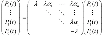
P t′ = −λ P t +αP₋ t + +⋯ α₋Pt +αP t P t −λ (6) Equation (6) can also be represented by matrix, as follow:

1

1 1 1

0 0

( ) ( )

( ) ( )

( ) ( )

n n n

P t P t

P t P t

P t P t

λ λα λα

λα λ

′ ₋

    

    

  ₌  

    

    

−

 

   

⋯

⋮ ⋱ ⋱ ⋮ ⋮

⋱

We can obtain the equation Pn′( )t = QPn( )t , and the characteristic equation of the coefficient matrix P is

1

det(_P−λ′_E)= − −( λ λ′)n+ =0

, so −λ is a characteristic root of P. The solution of Fn+1(−λ)A =0 is an arbitrary constant vector. Furthermore, cA is a certain vector by the uniqueness of pmf and (4), and it won’t changed with the change of α α1, 2,⋯.

Considering an extreme case: if α1=1, then we have

* ( )

() ( , , , )

!

n t

t T

n

t

t e

te e

n t

λ

λ λ

λ − _λ − −

= ⋯

P

,

where *

( )

n t

P can be expressed as

2 1

1

* )

[

2!

)

0 0

0 (

( ) 0 0

0 0

0

0 1

(

0 ] !

n

n

n n

t

n t

E t

t c e t

n

λ

λ λ

λ

− +

−

= + + +

 

  _{ }

  _{ }

   

 

 

 

 

 

 

+

⋯

⋯ ⋱ ⋮

I I

P

A

By Lemma 3 and In is an n-dimension identity matrix.

) ) ( ( 1 1 ! ! n n t t t t t t t e n n c e

t te

e λ λ λ λ λ λ λ λ λ − − − −          =                        ⋯ ⋮ ⋱ ⋱ ⋮ ⋱ A

Solve this system of equation, we obtain

(0,..., 0,1)T

cA= .

Using the expression of particular solution to solve

(−λ)c ,⋯, n(−λ)c

F A F A, we can get

1 1 1 1 1 1 1 1 2 1

1 2 1

( ( ,...,

0

0 0

( ) 0

0 0

1 0

) , 0)

n n n n n n T c

c N N

α α α

α α

λ λ α

α

α α α

λ λ − −               − = _{ }             = + = ⋯ ⋱ ⋮ ⋮ ⋯ F A

N N + + N A

1 1 2 2 2 2 2 1 2 2 2 2 2 2 2 1 2 0 0 0 0 0

( ) 0 0

0

0 0

( ( ,..

1 0

., , 0, 0

) ) n n n n T N c N N N c N λ λ λ λ

α α α

−               − = _{ }            + =  ⋯ ⋱ ⋮ ⋮ ⋯ F A

N N + + N A =

，……， 2 1 2 2 1 2 (

( ,..., , 0, , 0)

( ) ) ( ) ) ( , , ,

0 , 0)

(

i n i

n

n n n

n

n n T

n i

i n i T

i i n N N c c c c N

λ α α α

λ α α

λ λ α λ λ − + − + = = = ⋯ ⋯ ⋯ ⋯ ⋯

F A N N + + N A

=

F A N N + + N A

According to Lemma 3, it will be noticed that the unique solution of (6) is as follow:

1 2 1 1 1 2 2 0 2 (

(0,..., 0,1) ( ,..., , 0) ( ,..., , 0, 0)

( (

( ,.

( ( ), , ( ), ( ))

)

.., , 0, , 0) ( ,

[

2!

) )

]

! 0,..., 0) !

T

T n

i n

n T n T

n i T n T

i i n

t

N N N N

N N

P t P t P t

t t

t t

e

i N n

λ

λ λ

λ λ −

= + +

+ + ⋯ + +

⋯

⋯ ⋯

By the definition of N_in, to show (1), we only consider the first row of Pn( )t .

3.4. Matrix Differential Equation

According to the proof in system of differential equation method, we have the identity in matrix form

( ) ( )

n′t n t

P = QP ,

thus 2 1 2 0 ( ) ) ) ! ( ( n m m n m t n t m

t e α α α λ

∞

=

− + +

= Q =

∑

I N N +⋯+ N

P C C

Let t→0, hence we have the initial condition:

0 0

(0, , 0,1)T lim n( ) lim t

t→ t t→ e

= = =

⋯ Q

P C C

By Lemma 4, we have

0 1

0 1 1

1

1

, N 0 1

( ) ( ) ! ! ( ) ( ) , ! ! ! ! n n i i n n i m m i i

k k k m nm

l

n n

k k k m k n

k ik nk l

m m

k k k m

α

α α α

= + + + = ∈ + + + + = − + ₋ = + + − _{+ +}

∑

∑

⋯ ⋯ ⋯ ⋯ ⋯ ⋯ ⋯ I N I E N N 0 0

0 0 1 1 1 2 1 1 2 1 1 2 1

0 , N 0

1 2

2

1 2

1 , N 1 2

1

( 1) ( )

[ ! ( ) ] ! ! ( ) ! ! ! ( ) n i i n n n n n n i i n k k

k k k k m k k ik nk l

k k k

k k l n

n

k k k

k k t l n

m k k k m k n

k ik nk l nm n l t k t k k t e k t k k λ λ

α α α _λ

α α α _λ

∞ = + + + = ∈ + + + + = + + + + − = + + = ∈ + + + + = = − ⋅ = =

∑

∑

∑

∑

⋯ ⋯ ⋯ ⋯ ⋯ ⋯ ⋯ ⋯ ⋯ ⋯ ⋯ ⋯ N C N C P 1 . n n l=

∑

∑

Because ofN Cl =(1, 0,⋯, 0)T, if we choose the first row ofP_n( )t , (1) is easy to be prove by the statement above.

The following two methods is the derivation of the pmf by pgf.

3.5. Faà di Bruno Formula

Firstly, we give two approaches to prove Theorem 2. Similar to the binomial distribution approximate Poisson distribution, as well as the building method in the Section 3.4, it is easily to obtain the parameter limited conditions of multinomial distribution approximate to DCP by pgf:

1

1 1

( 1)

1 1

( ) lim [(1 ) ]

lim [1 ( )]

k i i i i i N i i Np t i i N t s i N i i N i i

P s p p s

t

s e

N

α λ

λ α

λ _{α α} ∞=

∞ ∞ = _{= =} →∞ − ∞ ∞ →∞ _{= =} ∑ = − + = + − =

∑

∑

∑

∑

.

Or by defining the pgf asP t s( , )= i ₀P t si( ) i ∞

=

∑

, substitute

to (5) we can get the expression as an ODE

1

( , )

=[ i( i 1)] ( , )

I Q t s

t s Q t s

t λ α

∞

=

∂ ₋

∂

∑

.

Thus we have

1 ( 1) ( , ) i i i t s

Q t s ce

λ ∞α

= −

∑

= .

Let s=1, by the definition of pgf, we know that (2) is the solution of the ODE above.

pmf of DCP. By the pgf of DCP, we have

1 ( )

0 1

{( !) [ ( i 1)] j }kj ( )kj

i _s i

i

j α λt s α λt

∞ −

=

= − =

∑

，

1 ( 1) ( )

0

[ t i i si ]i t

s

eλ α eλ

∞ = − − = ∑ = . 1 1 2 1 2 1 2 ( 1) 0 1 2 , N 1

1 2 2 1 ( ) [ ] ! [ ( ) ] ! ! ! i i i n n u n t s n _s k k k i t n

k k k i k n

k k nk n

n

n

i

n

P t e

n d k d t e k s k λ α λ

α α α _λ

∞ = − = − + + + = = ∈ + + + = ∑ → = =

∑

∑

⋯ ⋯ ⋯ ⋯

Let i running from 1 to n, and the Theorem 1 is proved.

3.6. Cauchy’S Integral Formula

Utilizing the relationship of Cauchy formula of higher order derivative and power series as well as formula (4), we have the pmf

1

0 0

0 0 1

1 1 1 1 2 1 2 1 0 1 1

0 , N 0

1 1 1 1 ( ) 2 ) 1 1 ( 2 !

1 1 ( 1) ( ) [ 2 ! ( ) ! ! ( 1 ) i i n i i n i n t tz

n _C n

m m n C m k k n C

k k k k m k

k ik nk

k k k n l l n z

P t e dz

i z

dz

i z m

t

i z k

z

t

t k k

λ αλ

π α α π λ π α λ α λ ∞ = − + ∞ + = ∞ + = + + + = ∈ + + + + = + + + ∞ = − + ∑ = + = − = ⋅

∫

∑

∫

∑

∑

∫

∑

⋯ ⋯ ⋯ ⋯ ⋯ ⋯ ⋯ + 1 1 0 1 1 1 1

, N 1 1 ] ( ) 1 1 ( )

2 ! !

n

n n

n i

i n

k l

k k k

k t

l n

n C

k k k m

l k n

k ik nk l

z dz

t e

z dz

i z k k

λ

α α λ

π + + − + + + + = ∈ + + + + = ∞ = =

∫

∑

∑

⋯ ⋯ ⋯ ⋯ ⋯ ⋯

By the results of complex integration, a is an internal point inC:

1, 1

1 1

.

0, 1 Z

2 C( )n ,

n dz

n n

i z a

π =  = ≠ ∈ − 

∫

When l=n, (2) is clearly.

3.7. Functional Equations

Wheni=0, the Chapman-Kolmogorov equation makes it

obviously that P t0( + ∆ =t) P t P0( ) 0(∆t).By Lemma 1, then

we have

0( )=e =1 ( ), ( 0) t

P ∆t − ∆λ − ∆ + ∆λ t o t λ> (7) When i=1, similarly, we have:

1( ) 0( ) (1 ) 1( ) 0( ).

P t+ ∆ =t P t P ∆ +t P t P ∆t (8)

By Lemma 1, 1( ) 1 ( 1 0)

t

P ∆ =t αte−λ α ≥ is clearly to see

by (7) and (8).

Continually, we have formulas below:

2 2

2 2 1 2

1

( ) [ ( ) ] (

! 0),

2

t

P t = α λt+ α λt e−λ α ≥ ⋯

1 2 1 2 1 1 2 1 2 , N ( ) ! ! ! ( ) n n n

i i i

k k k

k k k t n n ik k n n t e k k P k

t α α α λ λ

=

+ + + −

Σ = ∈

=

∑

⋯ ⋯

⋯

Then we use mathematical induction method to prove that (2) is true.

Moreover, we have

( ), ( 1,

( ) 2, )

i t i t o t i

P ∆ =λα∆ + ∆ = ⋯ ,

and it is easy to see the parameters of DCP process.αi must

be nonnegative constant due toP_i(∆ ≥t) 0.

3.8. Compound Poisson Sum

DCP process X t( ) can be decomposed as

1 2 ( )

( ) _{N t}

X t = + + +Y Y ⋯ Y ,

where Y_i is i.i.d nonnegative integer-valued random

variables with P Y{ 1= j}=αj, and N t( )∼P(λt).

We first verify that the pgf is formula (2), by the conditional expectation and independence:

1 1 ( ) ( ) 0 ( 1) 0

E E( | ( ) ) ( ( ) )

( ) (E ) ! i i i

X t X t

n

n t t s

Y n n

s s N t n P N t n

t e

s e

n

λ λ α

λ ∞₌

∞ = − − ∞ = ∑ = = = = =

∑

∑

Hence, by independence, we can figure that

1 2 1 2 1 ( ) 1 1 1 2 1 2 , ( ) { } ( )

{ , 1, 2, , , }

! ( ) ! ! ! i i n n n

i i i

N t n i i k t n i

i i i i

i k k k

k k k t n

n ik n k N

P t P Y n

t e

P k i n ik n k N

k

t e

k k k

α λ

λ

α λ

α α _{α λ}

= =

−

=

+ + + −

Σ = ∈

= =

= = Σ = ∈

=

∑

∑

⋯ ∼ ⋯ ⋯ ⋯

3.9. Sum of Weighted Poisson

DCP process X t( )can be decomposed as

1 2

( ) ( ) 2 ( ) i( )

X t =Z t + Z t + +⋯ iZ t +⋯,

where Z ti( ) is independent of each other, and

( ) ( )

i i

Z t ∼P λ αt .

We first verify that the pgf of X t( )is formula (3), by the conditional expectation and independence:

1 1 ( ) ( ) ( ) 0 ( 1) (s 1) 0

E E E( )

. i i i i i i i i

iZ t Z t

X t i

i

t s

t

i

s s s

e e λ α λ α ∞ = ∞ = ∞ = − ∞ − = ∑ ∑ = = = =

∏

∏

1 2

1 2 1

1

1

1 2 1 2 ,

( ) { ( ) }

( )

{ , 1, 2, , , }

!

( ) .

! ! !

i i

n

n n

i i i

n

n i

i

k t

n i

i i i i

i

k k k

k k k t n

n ik n k N

P t P iZ t n

t e

P k i n ik n k N

k

t e

k k k

α λ

λ

α λ

α α _{α λ}

= =

−

=

+ + + −

Σ = ∈

= =

= = Σ = ∈

=

∑

∑

⋯

∼ ⋯

⋯ ⋯

Remark 3. The expectation of DCP processX t( ) is

1 1

E ( )X t = ΣE[ _i∞₌iZ_i]= Σ_i∞₌iα λ_i t.

E ( )X t is finite，iff 1 i iαi

∞ =

Σ < ∞ . By independent

increments property，

E{ ( ) ( ) ( ) ( ), } 0 E{ ( ) ( ), }

( ).

X t X s X s X s X s X s

X s

τ τ τ τ

− + ≤ = + ≤

=

1

( ) i i

X t − Σ∞₌iα λt satisfies the definition of continuous- time martingale,

E( X t( )) < ∞; E(X t( ) { ( ),X t τ≤ ) =s} X s( ), (∀ ≤s t).

Hence, X t( ) i1iα λi t

∞ =

− Σ is called discrete compound

Poisson martingale.

The variance of discrete compound Poisson process

( )

X t is

2

1 1

D ( )X t D[ i iZi] i iα λi t

∞ ∞

= =

= Σ = Σ .

D ( )X t is finite, iff i1i2αi

∞ =

Σ < ∞ . Hence, X t( ) is a square-integrable martingale.

Definition 3. (Square-integrable martingale,[27] p59) A square-integrable martingale {M t( )}_t≥0 such that

(

2

)

E [M t( ) −M s( )] | {M( ),τ τ ≤s} = −t s, (0≤ ≤s t) is called a normal martingale.

The compensated and rescaled process

1 2 1

( )

( ) i i

i i

i X t

M t t

i t

α λ α λ

∞ = ∞

=

− Σ Σ

≜

is a normal martingale (See Chapter 2 of [27]).

3.10. Recursive Formula

We begin by defining the indicator function

1

0 , 0

( )

, 0

j

x j

g x

j− x j

≠ ≠



=

= ≠



.

Then,∀ ∈k R n, ≥1, by the compound Poisson sum in Section 3.8, it follows that

0 ( )

1

1 1

1 1

1 1 1

( ) { ( ) } ( ) ( ( ) ) E[ ( ) ( ( ))]

( )

E[( ) ( ( ))] E[ ( ( ))]

!

( )

E ( )

( 1)!

( )

n n n

i

k t N t

i n n

i k

k t

n k

j n i k

k j i

n j j

k

P t P X t n ig i P X t i X t g X t

t e

Y g X t k Y g X t

k

t e

j t g Y j Y j

k

P t

j t

n

λ

λ

λ

λ α λ

α λ

+∞

=

− ∞

= =

− −

∞ −

= = =

−

= = = = =

= =

= + =

− =

∑

∑

∑

∑∑

∑

1

1 1 1

( )

( )

( 1)!

k t

n n

j n j

j j

t e t

j P t

k n

λ

λ − − λ _α

∞

−

= = =

= −

∑

∑

∑

and

( )

0

1

( ) { 0} { ( ) 0}

N t

t i

i

P t P Y P N t e−λ

=

=

∑

= = = = .

By using the recursive formula, and using mathematical induction method, it is clearly to get equation (6).

3.11. Convolution

According multinomial distribution expansion formula, compound Poisson sum property and Lemma 4 we get

1

1 1

0

0 1

2

1 2

0

1

, 1

{ ( ) } { ( ) ( ) } { ( ) }

( )

{ }

!

1 ( )

{ ( ) }

! !

! !

n

n u

i

i t i

k i k

n i t

i n

i

k k

n

k k i k n

k

P X t n P X t n N t i P N t i

t e

P Y n

i

t e

P p s p s

n s i

p p

k k

λ

λ

λ

λ

∞

=

− ∞

= =

− ∞

=

+ + = ∈ +

= = = = =

= =

∂

= + +

∂

=

∑

∑ ∑

∑

⋯ ⋯

⋯

⋯ ⋯

N

1

0

( ) n ,

u n

k k t i

uk nk n

t eλ

λ

∞

+ + − =

+ ++ =

∑

∑

⋯

where

1

{ }

i

k k

P Y n

= =

∑

is pmf of ith convolution of Yk.

3.11. Remark of the Methods

Arguing from the Chapman-Kolmogorov equation, Whittaker [33] obtained the difference differential equation relating toP tn( ), solving one by one, he gave the first 5 probability expressions of

( )( 0,1, 2,3, 4)

n

P t n= .

Janossy [17] directly solve the Chapman-Kolmogorov equation to get the expression of P tn( ), it shows that the superimposition condition in the definition of DCP process are unnecessary. Luders[24] name it Pollaczek-Geiringer distribution in memory of these two people's finding, and derived it by the method of sum of weight Poisson. Hofman [16] derive the expression of P tn( ) by the use of Faà di Bruno formula, from the pdf of P tn( ) . Adelson [1] differentiate pgf of DCP distribution for several times and obtained the recurrence relation of pmf.

discrete compound Poisson distribution. Among ten approaches, the system of differential equation, convolution, Matrix differential equation, Cauchy’s integral formula are

original works, the other methods give a detail and vivid

proof from other works.

Let α1=1 in DCP distribution, except for method of

compound Poisson sum, sum of weight Poisson and convolution, we obtain seven approaches to prove the pmf of Poisson distribution.

When it comes to parameter estimation of DCP, see [18] and [34].

4. Probabilistic Number Theory

In the probabilistic number theory, prime divisors of integers and the distribution of primes in short intervals have properties of Poisson distribution under some condition. The detail results are in this theoretical research papers: [15], [11], [8], [28] and [13]. Let f m( )be a real-valued arithmetical function whose domain is positive integer {1, 2, }⋯ . We say that strongly additive functions satisfies the following restriction.

(i). f m( + =n) f m( )+ f n( ) whenever ( , )m n =1. (ii). f p( k)= f p( ) for all prime p and k≥1.

For example, let f m( ) be the number of prime divisors of m. And the additive functions just satisfy (i).

Then we have the following results due to Bekelis [3]. In Bekelis’s work, he give the necessary and sufficient conditions for the weak convergence of the distribution functions of strongly additive functions to the finite Poisson law convolutions.

Theorem 4: Let f mx( ), (x≥1) be a strongly additive

function depend on x. Defined the pmf of u by

(

( ) )

x x

v f m =u

[ ]

1

( ( ) ) #{ : ( ) }

x x x

v f m m x f m

x

u = ≤ =u

=

Let functions f mx( ) on each prime number p is values from the nonnegative integer set

1 2 1 2

{0, ,c c ,⋯, }, 0c_r < <c c <⋯<c_r. If

, ( ) 0

, ( ) 0

, ( )

1 ln

lim max 0; lim 0; ln 1

lim , ( 1, , ),

x _x

x i

x p x f p x

p x f p

i x

p x f p c

p

p p x

j r

p λ

→∞ ≤ ≠ →∞ _{≤ ≠}

→∞ _{≤ =}

= =

= =

∑

∑

⋯

(9)

then the limited pgf of vx(f mx( )=u)is 1 ( 1)

0

( ) , ( 1)

lim ( ) .

r _ci

i

i s

u x x

x u

v f m us e =λ s

∞ ₋

→∞ =

∑

= = ≤

∑

Hence u∼CP(⋯,λ1,⋯,λ2,⋯,λr).

Theorem 5: Let strongly additive functions f m_x( ),

(x≥1) be as described above, and the limited pgf of

( ( ) )

x x

v f m =u is

1 ( 1)

0

( ) , ( 1)

lim ( ) ,

r ci

i

i s

u x x

x _u v f m us e s

λ

=

∞ ₋

→∞ =

∑

= = ≤

∑

if numbers cj, (j=1, 2,⋯, )r are linearly independent over the field ℚ, then conditions (9) are satisfied (i.e., they are necessary and sufficient in this case).

The proof of Theorem 4 and Theorem 5 is in [3], then rewrite the corresponding characteristic function to the pgf of vx(f mx( )=u).

Šiaulys [28] prove that if f is a strongly additive function on prime number with f p( ) {0,1}∈ , then f is Poisson distributed on the integers under the condition that

1

r= in (9). This is a special case of Theorem 4.

Numerical example: Let x( ) x( )

p m

f m =

∑

f p be the sum

of fx( )p under condition that p m, where

4 2

2 4

0, ln ln (ln ln )

( ) 1, ln ln (ln ln )

2 (ln ln ) (ln ln )

x

p x or p x

f p x p x

x p x

< >

 

= ≤ ≤

 _{≤ ≤}



Bekelis [3] obtain

1 2

( ) 1 ( ) 2

1 1

lim ln 2, lim ln 2

x x

x x

p x p x

f p f p

p p

λ λ

→∞ _≤ →∞ _≤

= =

=

∑

= =

∑

=

.

Thus u approximate to Hermite distribution with pmf

1 2

[ ] ₂ [ ]

2 2

1 )

0 (

2

0

1 (ln 2) ( )

( 2 )! ! 4 ( ! ! )

2 (

)

x x

u u

u i i u i

i i

e u

u i i u

v f m

i i

λ λ

λ − λ −

= =

− +

=

− −

≈

∑

=

∑

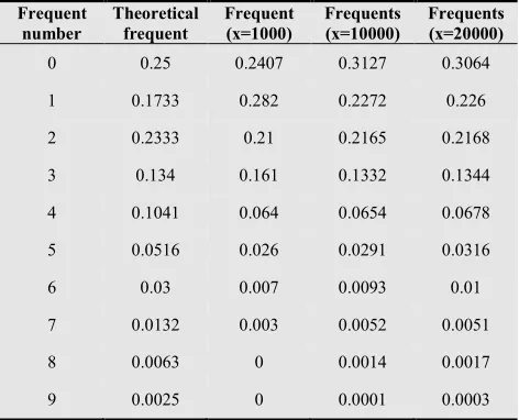
Table 1. Frequent when x=1000, 10000, 20000

Frequent number

Theoretical frequent

Frequent (x=1000)

Frequents (x=10000)

Frequents (x=20000)

0 0.25 0.2407 0.3127 0.3064 1 0.1733 0.282 0.2272 0.226 2 0.2333 0.21 0.2165 0.2168 3 0.134 0.161 0.1332 0.1344 4 0.1041 0.064 0.0654 0.0678 5 0.0516 0.026 0.0291 0.0316 6 0.03 0.007 0.0093 0.01 7 0.0132 0.003 0.0052 0.0051 8 0.0063 0 0.0014 0.0017 9 0.0025 0 0.0001 0.0003

In order to obtain equality, we would have to let

ln lnx→ ∞ in some fashion. The convergence rate is very

slow. Since limited conditions in computer, we can’t calculate the larger value of xin this paper by Matlab.

Theorem 6. (Erdos-Wintner, 1939): A necessary and sufficient condition for a real additive function f m( ) to have a limiting distribution is that the following three series converge simultaneously for at least one value of the positive real numberR:

2

( ) ( ) ( )

1 ( ) ( )

; ;

f p R f p R f p R

f p f p

p p p

> ≤ ≤

∑

∑

∑

When these conditions are satisfied, the characteristic function of the limit law is given by the convergent product

1 ( )

0

( ) [ v(1 ) i f pv ]

v p

p p eτ

ϕ τ ∞ − − =

=

_∏

∑

−

The limit law is necessarily pure. It is continuous if, and

only if 1

( ) 0

f p

p−

≠ = ∞

∑

.

For further explanation for Erdos-Wintner theorem, see [9] and [29]. Using Erdos-Wintner theorem, we have the following theorem

Proposition 1. In the Erdos-Wintner theorem, if

( ) 0

1

f p≠ p

< ∞

∑

and f m( )takes non-negative integer value,

then ϕ τ( )approximate to a discrete compound Poisson distribution with pgf

1 ( ) 1 ( ) 0 1 ( ) 0

(1 )

( ) , ( 1)

v

v f p

f p v f p

p p s p

P s e s

∞ _{− − −}

≠ = − − ≠

∑ ∑ ∑

= ≤

Proof: Rewrite the characteristic function ϕ τ( ) to the

pgf, and notice that 1 x

x e

+ ≈ for a sufficient small

1 ( )

1

(1 ) v 1

v f p

v

x p p s

∞

− −

=

=

∑

− ≪ , then

1 ( ) 1 1

1 ( ) 1 ( ) 0 1 ( ) 0

1 ( ) 1

1

1 ( ) 1

1 (1 )

(1 )

( ) [(1 (1 ) ] [(1 (1 ) ]

.

v

v

v

v f p

v

v

v f p

f p v f p

v f p

v p

v f p

v p

p p s p

p

p p s p

P s p p s p

p p s p

e

e

∞

− − −

=

∞

− − −

≠ = ≠

∞

− − −

= ∞

− − −

=

− −

− −

∑

∑ ∑ ∑

= + − −

= + − −

≈

=

∑

∏

∑

∏

∏

5. (S,s) Inventory Policies under

Stuttering Poisson Demand

Considering the sales of an enterprise, the interval is a week, and the week sales are random. Then management decides whether to order goods to satisfy the needs of next week. One of the most simple

inventory strategy is (s,S) inventory policies: the lower bound of s, the upper bound of S .When the inventory at weekend is less than s ,order stocks to reach S, otherwise, don’t order.

In fact, we need to take ordering fee, storage fee, out of stock payment and purchase fee into account and then formulate an inventory strategy to minimize the total average cost. Generally speaking, the arrival of demand satisfies the property of discrete stationary independent increments process. But a customer may purchase the same goods more than one once, so we can assume that the random demand satisfies stuttering Poisson distribution.

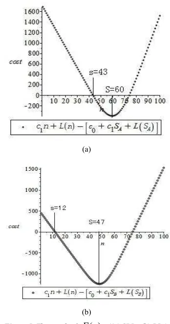
Suppose that each ordering fee is c0, the bid of each

good is c₁, the storage fee of each good is c₂ and the loss of each good that out of store is c3. In order to

facilitate computation, we assume that the weekly sale

r

is a nonnegative integer-valued random variable, and the pmf is p r( ). If the stock in the end of the week is

x

,

order quantity is

u

, so the stock at the beginning of the

next week isx u+ , storage capacity in every week

isx u+ −r.

According to (S, s) inventory strategy, ifx≥s, order

quantity u=0 ; if x<s , u>0 and the constraint isx u+ =S. Now we determine (S, s) through figuring out the minimum of the average cost. The storage cost and the expected value of back-order loss in a week is

2 ₀ 3

( ) x( ) ( ) ( ) ( )

x

L x =c

∫

x−r p r dr+c

∫

∞ r−x p r dr

The average cost in a week is the sum of order cost, bid cost, storage cost and the back-order loss,

0 1 ( ), 0

( )

( ), 0

c c u L x u u

J u

L x u

+ + + >



=

=



Determination of S:

Now we take the derivative and second derivative of the average cost function about

1 2 ₀ 3

2 3 ₀ 3 1

( )

( ) ( )

====( ) ( ) ( )

x u

x u

S x u _S

dJ u

c c p r dr c p r dr

du

c c p r dr c c

+ ∞

+ = +

= + −

+ − −

∫

∫

∫

LetdJ u( ) 0

du = , then we can solve that when S satisfies

3 1 0

2 3

( )

S c c

p r dr

c c

− =

+

∫

,

then,J u( ) reaches the minimum. Determination of s:

Then, determine the order number s according to x. If management decide to order some goods, and the number is u, sincex u+ =S , the total cost is

1 0 1( ) ( )

J = +c c S− +x L S