Data Reduction Influence on the Accuracy of Credit Risk Estimation Models
Ricardas Mileris, Vytautas Boguslauskas
Kaunas University of Technology
K. Donelaicio str. 73, LT-44309, Kaunas, Lithuania
e-mail: [email protected], [email protected]
Credits in banks have risk of being defaulted. The main purpose of credit risk estimation in banks is the determination of company‘s ability to fulfil its financial obligations in future. It is very important to have a proper instrument for the estimation of credit risk in banks because it reduces potential loss due to crediting reliable clients. Banks develop internal credit risk estimation models and various data analysis methods can be applied for this purpose. Statistical predictive analytic techniques and artificial intelligence can be used to determine default risk levels. Banks must also have data about clients from the activity in the past. To understand risk levels of credits, banks usually collect information about borrowers. Financial ratios remain primary variables for predicting corporate financial distress. The principal financial ratios as variables for the analysis are indicators of company‘s financial structure, solvency, profitability and cash flow. Credit risk estimation models are based on the analysis of this data. Using these models it becomes possible to predict the default possibility of new clients. Credit risk estimation models in banks differ significantly in architecture and operating design. The main reason for these differences is that banks’ models are assigned by bank personnel and are usually not revealed to outsiders.
The object of this research is credit risk estimation models. The purpose of research is to develop credit risk estimation models and to evaluate an influence of input data reduction on credit risk models accuracy. Two methods were applied in this research: the analysis of scientific publications about estimation of credit risk and the analysis of developed in this research credit risk estimation models performance.
Analyzing financial data of Lithuanaian companies three initial credit risk estimation models were developed wherein these data analysis methods were applied: discriminant analysis (DA), logistic regression (LR) and artificial neural networks (ANN) - multilayer perceptron. 60 financial rates of companies were analyzed. They were calculated from the financial reports of Lithuanian companies for 3 years. The variable selection for the DA model was accomplished applying the analysis of variance (ANOVA) and Kolmogorov-Smirnov test. The variable selection for the LR model was accomplished applying ANOVA. The actual variables for credit risk analysis in ANN model were selected by network according to their ranks of importance. The classification accuracy of models was evaluated by the correct classification rate (CCR). The highest classification accuracy was reached by LR model,
which classified 97% of companies correctly. ANN model correctly classified 95.5%, DA model – 84% of companies.
Further situation was analyzed where 60 initial variables were reduced applying factor analysis and the changes in classification accuracy of models were estimated. The number of factors to retain were calculated by the Kaiser criterion ant the scree test. After the factor analysis the 6 new credit risk estimation models were developed applying the same data analysis methods: DA, LR and ANN. By every method 15 and 6 new variables obtained from the factor analysis were analyzed. The research has shown that the new 15 variables extract 89.37% of variance from initial variables. Analyzing these variables, the percent of correctly classified companies mostly decreased in ANN model (-14.6%). The classification accuracy of other models decreased from 2.0% to 7.1%. If an analyst includes into credit risk estimation only 6 new variables, which extract 63.92% of variance from initial variables, the highest decrease in classification accuracy will also be in ANN model (-15.7%).
Keywords: artificial neural networks, credit risk, discriminant analysis, factor analysis, logistic regression.
Introduction
Credit risk analysis has recently emerged as a necessity to help banks understand the importance of this risk and plan the appropriate countermeasures in advance. Usually such analysis is based on a number of indicators (parameters) that quantify the clients on which a bank designs credit risk measurement instruments.
Therefore there is no absolutely correct ways of estimating credit risk level for all situations. Different models allow to make the best decision in concrete cases. Under the conditions of objective existence of risk and connected with it financial and other losses, there is always a need for a certain mechanism which would allow to measure credit risk while making decisions.
The object of this research is credit risk estimation models.
The purpose of research is to develop credit risk estimation models and to evaluate the influence of input data reduction on developed credit risk models accuracy.
The methods of the research:
1. Analysis of scientific publications.
2. Analysis of credit risk estimation models performance.
Credit scoring models and their classification techniques are under examination in this study. This study explores the performance of credit scoring models using traditional and artificial intelligence methods: discriminant analysis, logistic regression and artificial neural networks. Experimental studies using real financial data of Lithuanian companies have to demonstrate the influence of data reduction on models classification accuracy.
The purpose of credit scoring models
In recent years banking activity is increasing in many countries. Foreign banks entered the emerging markets to expand their business in various countries (Voinea, Mihaescu, 2008). Credits to private and public sectors increase money supply there, that influence investments, consumption and economic growth (Teresiene, Aarma, Dubauskas, 2008). Companies often need credits and their successful activity is one of the most important economics growth factors having the basic impact on the general development of the country’s economy and social stability, creation of new work places (Tamosiunas, Lukosius, 2009).
The empirical findings of many studies suggest that bank‘s specific characteristics, in particular loans intensity, credit risk, and cost have positive and significant impacts on bank performance (Sufian, Habibullah, 2009). The goal of every bank is to achieve the highest profit at the lowest capital price. It determines the need of shareholders to operate using debt as much as possible. Long-term profitable activity of bank using high level of debt shows competence of management team (Gimzauskiene, Valanciene, 2009). The use of statistical analysis methods and information technologies in banks in pursuance of improving work processes is one of the most important opportunities of the application of these technologies in risk management, work and communication processes (Gatautis, 2008).
Bankruptcy predictions and solvency measurements have become important research topics for scientists and credit analysts. As the world’s economy has been facing several challenges during the past decades, more and more companies are addressing the problems of insolvency. Within the current context of dynamic changes in business environment the theory and practice of financial management face a question: which method of evaluation of company’s financial stability and credit risk to use (Koleda, Lace, 2009).
Categories of risk and return are becoming increasingly important in banks business process. The knowledge of risk indices allows to manage risk properly. The well provided risk management methods let make more reasonable and adequate managing decisions
(Vlasenko, Kozlov, 2009). Bank cannot use primitive risk estimation models because proper risk management ensures the bank’s profit (Jovarauskiene, Pilinkiene, 2009). The proper decisions lead to a higher level of efficiency. The quality of decisions may be perceived as a function of imperatives (requirements, regulations, orders, sophistication and knowledge) that is based on information needed for decision making (Gudonavicius, Bartoseviciene, Saparnis, 2009). Typical problems of risk estimation in banks are: how to decide which information is valuable and which one is useless, finally, how to assess the quality of the usable information (Ruzevicius, Gedminaite, 2007).
Credit scoring is a very important task for lenders to evaluate the loan applications they receive from clients. Credit scoring models are used to model the potential risk of loan applications, which have the advantage of being able to handle a large volume of credit applications quickly with minimal efforts, thus reducing operating costs, and they may be an effective substitute for the use of judgment among inexperienced loan officers, thus helping to control bad debt losses (Ince, Aktan, 2009). Information technology applications that support decision-making processes and problem solving activities have proliferated and evolved over the past few decades. These systems were further enhanced with components from artificial intelligence and statistics. Intelligent decision-support using advanced decision and optimization technologies are becoming increasingly important in banks and business management (Sakalauskas, Zavadskas, 2009). Banks use statistical methods such as discriminant analysis, linear probability models, probabilistic analysis, artificial intelligence methods, expert systems, artificial neural networks, genetic algorithms, etc., to identify credit risk, (Chen, Li, 2009).
The objective of credit scoring models is to decide whether or not to grant credit to an applicant. The majority of credit scoring models assign credit applicants to either a “good credit” group, which is likely to repay a financial obligation, or a “bad credit” group, with a high probability of defaulting on the financial obligation and hence their application should be denied. Therefore, credit scoring models basically belong to the field of classification problems (Mavri, Angelis, Ioannou, Gaki, Koufodontis, 2008). The accuracy of their estimations over a period of time is very important for financial results of a bank.
Credit scoring modeling has become a core component in risk management systems in banks and financial institutions. In fact, banks are prompt to develop or buy such models in order to make the whole procedure of evaluating credit applications faster, easier and more accurate.
Factor analysis as a data reduction method
The main applications of factor analytic techniques are:
x to reduce the number of variables;
x to detect structure in the relationships between variables, that is to classify variables.
a single underlying factor that is responsible for the observed correlations (Li, Zhao, Ma, 2008). According to Oreski and Peharda (2008), the central aim of factor analysis is the orderly simplification of several interrelated measures using mathematical procedures. Traditionally, a factor analysis has been used to explore the possible underlying structure in a set of interrelated variables without imposing any preconceived structure on the outcome (Oreski, Peharda, 2008).
If the information on each variable Xiis decomposed to represent the linear combination of various information factors, then:
Xi = ai1F1 + ai2F2 + … + aikFk + diUi (1) where F1, F2, …, Fk – the common factors, which reflect certain information common in many variables;
ai1,ai2, …, aik– the common factor loads;
Ui – a special factor, which is only related to the variable Xi, indicating a certain special character of this variable;
di – load of special factor.
The common factor is expressed by the linear combination of variables under investigation:
Fj = ȕj1X1 + ȕj2X2 + … + ȕjnXn (2) ȕji – factor score coefficients;
Xi – variables (Lu, Han, Gao, Cao, 2006).
Factor score coefficients are used to compute the factor scores. Factor scores can be estimated as new variables of individual cases. These factor scores are particularly useful when there is a need to perform further analysis involving the factors that were identified in the factor analysis. Factor scores in the next steps of analysis reduce the data and the research on the original problem can be continued (Chen, Li, 2009).
Each common factor is extracted according to the magnitude of variance contribution of each factor. The common factors extracted in this order are called the 1st principal factor, the 2nd principal factor, …, the kth principal factor respectively (Lu, Han, Gao, Cao, 2006).
The number of factors is an arbitrary decision. However, there are guidelines that seem to yield the best results. First, we can retain only factors with eigenvalues greater than 1. This is like saying that, unless a factor extracts at least as much as the equivalent of one original variable, we drop it. This criterion was proposed by Kaiser (1960). Also the graphical method can be applied - the scree test. It was proposed by Cattell (1966). We can plot the eigenvalues in a line plot. Cattell suggests to find the place where the smooth decrease of eigenvalues appears to level off to the right of the plot (Oreski, Peharda, 2008).
Developed credit risk estimation models
The essence of models was to classify companies into 2 groups:
x Group 1: reliable companies with low possibility of default.
x Group 2: not reliable companies with high possibility of default.
Data sample of this research consisted of 100 Lithuanian companies. In this sample 50 companies operated successfuly and 50 companies bankrupted. Every company was characterized by 20 financial ratios of 3 years:
1. Liquidity ratios: 1.1. Curent ratio; 1.2. Quick ratio; 1.3. Cash to current liabilities; 1.4. Working capital to total assets.
2. Profitability ratios: 2.1. Gross profitability; 2.2. Net profitability; 2.3. Net profit to total assets.
3. Leverage ratios: 3.1. Total liabilities to total assets; 3.2. Total debt to equity; 3.3. Long term debt to equity; 3.4. Equity to total assets.
4. Activity ratios: 4.1. Sales to total assets; 4.2. Sales to long term assets.
5. Other ratios: 5.1. Cash to total assets; 5.2. Current assets to total assets; 5.3. Unappropriate balance to total assets; 5.4. Working capital to sales; 5.5. Activity profit to total assets; 5.6. Activity profit to sales.
The financial reports of 3 years were analyzed, so overall 60 ratios are available for analysis.
Three initial credit risk estimation models were developed wherein these data analysis methods were applied:
1. Discriminant analysis (DA). 2. Logistic regression (LR).
3. Artificial neural networks (ANN).
1. Discriminant analysis (DA). The classification functions allow to determine which group each company most likely belongs to. There are 2 classification functions in the model as there are 2 groups of companies (reliable and not reliable). When analyzing data each function computes the classification score for the groups of reliable and not reliable clients:
fj = Įj + ȕj1x1 + ȕj2x2 + … + ȕjnxn (3) where j – number of the respective group;
Įj – the constant for the j group;
ȕji – the weight for the variables in the computation of the classification score for the j group;
xi – the observed value of each variable for the respective company.
Result fj is the classification score. Having computed the classification scores, we classify the bank client as belonging to the group for which it has the highest classification score fj.
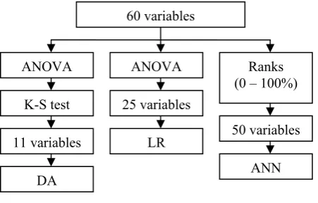
Variable selection was accomplished applying the analysis of variance (ANOVA) and Kolmogorov-Smirnov (K-S) test. The purpose of ANOVA was to test for significant differences between means. The variables were rejected which means in the groups of reliable and not reliable clients do not differ significantly. The Kolmogorov-Smirnov one sample test for normality is based on the maximum difference between the sample cumulative distribution and the hypothesized cumulative distribution. This test allowed to verify if the variable has the normal distribution. If the D statistic is significant, then the hypothesis that the respective distribution is normal should be rejected. These variables were not included in the credit risk analysis. So after variable selection 11 variables were analyzed by the discriminant analysis model (Figure 1).
fitting data to a logistic curve. In credit risk estimation the event is company‘s default.
To model the relationship between creditworthiness of a client and its financial information, the bank can assume that the possibility of default (p) depends on the company‘s financial ratios (xi) as follows:
n n n n x x x x x x e e
p D E E E
E E E D ... ... 2 2 1 1 2 2 1 1
1 (4)
where Į is the intercept and ȕ1, ȕ2, ..., ȕn, are the regression coefficients of variables x1, x2, ..., xn respectively. The above model (4) is called a logistic regression model (Xi, Lin, Chen, 2009).
All p values depend to range [0; 1]. They reflect enterprise‘s possibility of default from 0 to 100%. Because classification of clients was implemented into two groups the classification threshold was set to 0.5.
The variable selection for this model was accomplished applying ANOVA. After analysis of variance 25 variables were used in logistic regression model (Figure 1).
3. Artificial neural networks (ANN). The multilayer perceptron (MLP) network was developed to solve bank clients classification problem. MLP network consists of a set of source nodes forming the input layer, one or more hidden layers of computation nodes, and an output layer of nodes. The input signal propagates through the network from one layer to another. The perceptron computes a single output from multiple inputs by forming a linear combination according to its input weights and then possibly putting the output through some nonlinear activation function. Neural network learns by appropriately changing the internal connection weights (Purvinis, Sukys, Virbickaite, 2005).
The actual variables for the credit risk analysis were selected by a network according to their ranks of importance. The range of ranks is from 0% (the variable is not important) to 100% (the variable is very important). 10 variables with ranks of 0% were rejected and 50 variables were used in this model (Figure 1).
Figure 1. Variable selection for initial models
The classification accuracy of models was measured by the correct classification rate (CCR). It is the proportion of correctly classified companies:
CCR = (TP+TN)/N (5)
where TP (True Positive) – correctly classified not reliable companies;
TN (True Negative) – correctly classified reliable companies;
N – number of companies analyzed.
The highest classification accuracy was reached by LR model, which classified 97% of companies correctly. ANN model correctly classified 95.5%, DA model – 84% of companies (Figure 2).
84 97 95.5 0 20 40 60 80 100
DA LR ANN
%
Figure 2. The correct classification rates (CCR) of developed models
Further situation was analyzed where 60 initial variables were reduced applying factor analysis. It was important to estimate the changes in classification accuracy of models.
Data reduction applying factor analysis
Factor analysis was applied as a data reduction method to reduce the quantity of data analyzed by credit risk estimation models.
Numbers of factors to retain were calculated by:
x The Kaiser criterion.
x The scree test.
According Kaiser criterion, we can retain only factors with eigenvalues greater than 1 (Table 1).
Table 1 Eigenvalues and extracted variance
Value Eigen-value Total variance, % Cumulative eigenvalue Cumulative variance, %
1 11.69 19.49 11.69 19.49
2 7.83 13.05 19.52 32.54
3 6.52 10.87 26.05 43.41
4 5.21 8.69 31.27 52.11 5 4.39 7.33 35.67 59.45 6 2.68 4.46 38.35 63.92 7 2.53 4.22 40.88 68.14 8 2.30 3.84 43.19 71.98 9 2.05 3.42 45.24 75.40 10 1.78 2.96 47.02 78.37 11 1.68 2.80 48.71 81.18 12 1.47 2.45 50.18 83.64 13 1.26 2.11 51.45 85.75 14 1.11 1.86 52.57 87.61 15 1.05 1.75 53.62 89.37
The variances extracted by the factors are called the eigenvalues. If a factor extracts less variance as the equivalent of one original variable, we reject it. Using this criterion, 15 factors (principal components) were retained.
Eigenvalues and extracted variance of factors after rotation Varimax normalized are shown in Table 1. In the second column of this table (Eigenvalue), we find the 60 variables ANOVA K-S test 11 variables DA ANOVA 25 variables LR Ranks (0 – 100%)
variance on the new factors that were successively extracted. The sum of the eigenvalues is equal to the number of variables (60). In the third column, these values are expressed as a percent of the total variance. As we can see, factor 1 accounts for 19.49 percent of the variance, factor 2 for 13.05 percent, and so on. The fourth column contains the cumulative variance extracted. The fifth column (Cumulative variance, %) indicates the cumulative percent of the total variance extracted by factors.
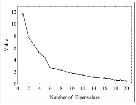
In order to accomplish the scree test, it is necessary to plot the eigenvalues in a simple line plot (Figure 3).
0 2 4 6 8 10 12 14 16 18 20
Number of Eigenvalues 0
2 4 6 8 10 12
Va
lu
e
Figure 3. Plot of eigenvalues
We find the point where the smooth decrease of eigenvalues appears to the right of the plot. This point (number of eigenvalues) is equal to 6. According to this criterion, 6 factors were retained in the sample.
Classification accuracy of credit risk estimation models after data reduction applying factor analysis
Owing to problems of missing values in some variables, it was necessary to exclude some companies from the analysis, such that data collection resulted in a total of 89 companies.
The 6 new credit risk estimation models were developed applying the same data analysis methods: discriminant analysis, logistic regression and artificial neural networks. By every method 15 and 6 new variables obtained from factor analysis were analyzed.
Table 2 Correct classification rates of models, %
15 variables 6 variables
Model
CCR Change CCR Change
DA 82.0 -2.0 73.0 -11.0 LR 89.9 -7.1 82.0 -15.0
ANN 80.9 -14.6 79.8 -15.7
The research has shown that the new 15 variables extract 89.37% of variance from initial variables. Analyzing these variables, the percent of correctly classified companies mostly decreased in ANN model (-14.6%). The classification accuracy of other models decreased from 2.0% to 7.1% (Table 2). If the analyst includes into credit risk estimation only 6 new variables, which extract 63.92% of variance from initial variables, the highest decrease in classification accuracy will be also in ANN model (-15.7%).
Conclusions
1. In this research credit risk estimation models were developed applying 3 data analysis methods: discriminant analysis, logistic regression and artificial neural networks.
2. The proposed models analyze the financial data of credit applicants and predict the future repayment behaviour for those who have been characterized as creditworthy and not creditworthy clients.
3. The influence of input data reduction by factor analysis on the classification accuracy of models was estimated. As the results of the factor analysis indicated, 15 variables extracted 89.37% of variance from initial variables. That reduced the classification accuracy of models from 2% to 14.6%. Also 6 new variables extracted 63.92% of variance from initial variables. That reduced the classification accuracy of models from 11% to 15.7%.
References
Abdou, H. A. (2009). An Evaluation of Alternative Scoring Models in Private Banking. The Journal of Risk Finance(1), 38-53.
Bensic, M., Sarlija, N., Zekic-Susac, M. (2005). Modelling Small-Business Credit Scoring By Using Logistic Regression, Neural Networks And Decision Trees. Intelligent Systems In Accounting, Finance And Management(13), 133-150. Chen, W. D., Li, J. M. (2009). A Model Based On Factor Analysis And Support Vector Machine For Credit Risk
Identification In Small-And-Medium Enterprises. Machine Learning and Cybernetics(2), 913-918.
Fantazzini, D., Figini, S. (2009). Random Survival Forests Models for SME Credit Risk Measurement. Methodology and Computing in Applied Probability(1), 29-45.
Gatautis, R. (2008). The Impact of ICT on Public and Private Sectors in Lithuania. Inzinerine Ekonomika-Engineering Economics(4), 18-28.
Gimzauskiene, E., Valanciene, L. (2009). Performance Measurement System In The Context Of Economics Changes.
Economics & Management(14), 33-42.
Gudonavicius, L., Bartoseviciene, V., & Saparnis, G. (2009). Imperatives for Enterprise Strategists. Inzinerine Ekonomika-Engineering Economics(1), 75-82.
Jovarauskiene, D., & Pilinkiene, V. (2009). E-Business or E-Technology? Inzinerine Ekonomika-Engineering Economics(1), 83-89.
Koleda, N., Lace, N. (2009). Development Of Comparative-Quantitative Measures Of Financial Stability For Latvian Enterprises. Economics & Management(14), 78-84.
Lieu, P. T., Lin, C. W., Yu, H. F. (2008). Financial Early-Warning Models on Cross-Holding Groups. Industrial Management & Data Systems(8), 1060-1080.
Liou, F. M. (2008). Fraudulent Financial Reporting Detection and Business Failure Prediction Models: a Comparison.
Managerial Auditing Journal(7), 650-662.
Liviu, V., Flaviu, M. (2008). What Drives Foreign Banks to South-East Europe? Transformations in Business & Economics(15), 107-122.
Lu, Y. L., Han, J. Y., Gao, W. H., Cao, S. G. (2006). Using Factor Analysis For Indentifying Latent Contributing Factors Of Customer Loyalty Evaluation Of Mobile Communication Enterprise. Machine Learning and Cybernetics, 1913-1917.
Mavri, M., Angelis, V., Ioannou, G., Gaki, E., Koufodontis, I. (2008). A Two-Stage Dynamic Credit Scoring Model, Based On Customers’ Profile And Time Horizon. Journal of Financial Services Marketing(13), 17-27.
Oreski, D., Peharda, P. (2008). Application of Factor Analysis in Course Evaluation. Information Technology Interfaces, 551-556.
Purvinis, O., Sukys, P., & Virbickaite, R. (2005). Research of Possibility of Bankruptcy Diagnostics Applying Neural Network. Inzinerine Ekonomika-Engineering Economics(1), 16-22.
Ruzevicius, J., & Gedminaite, A. (2007). Business Information Quality and its Assessment. Inzinerine Ekonomika-Engineering Economics(2), 18-25.
Sakalauskas, L., Zavadskas, E. K. (2009). Optimization And Intelligent Decisions. Technological and Economic Development of Economy, 15(2), 189-196.
Sufian, F., Habibullah, M. S. (2009). Determinants Of Bank Profitability In A Developing Economy: Empirical Evidence From Bangladesh.Journal of Business Economics and Management(10), 207-217.
Tamosiunas, T., & Lukosius, S. (2009). Possibilities for Business Enterprise Support. Inzinerine Ekonomika-Engineering Economics(1), 58-64.
Teresiene, D., Aarma, A., Dubauskas, G. (2008). Relationship Between Stock Market and Macroeconomic Volatility.
Transformations in Business & Economics(14), 102-114.
Ugurlu, M., Aksoy, H. (2006). Prediction of Corporate Financial Distress in an Emerging Market: the Case of Turkey.
Cross Cultural Management: An International Journal(4), 277-295.
Vlasenko, O., Kozlov, S. (2009). Choosing The Risk Curve Type.Technological and Economic Development of Economy,
15(2), 341-351.
Xi, R., Lin, N., Chen, Y. (2009). Compression and Aggregation for Logistic Regression Analysis in Data Cubes.
Knowledge And Data Engineering(21), 479-492.
Yu, L., Wang, S., Wen, F, Lai, K. K., He, S. (2008). Designing a Hybrid Intelligent Mining System for Credit Risk Evaluation. Journal of Systems Science and Complexity(21), 527-539.
Riþardas Mileris, Vytautas Boguslauskas
Duomenǐ apimties mažinimo Ƴtaka kredito rizikos vertinimo modeliǐ tikslumui
Santrauka
Paskolǐ teikimas yra viena iš rizikingiausiǐ bankǐ veiklos sriþiǐ, todơl labai svarbu turơti patikimą kredito rizikos vertinimo mechanizmą ir sugebơti tinkamai šią riziką valdyti. Kredito rizikos Ƴvertinimas yra vienas iš kredito suteikimo etapǐ. Pagrindinis kredito rizikos vertinimo tikslas yra nustatyti, ar verta suteikti kreditą. Bankai stengiasi sumažinti kredito riziką, nesuteikdami kreditǐ klientams, kurie turi mažiausias galimybes Ƴvykdyti prisiimtus finansinius Ƴsipareigojimus.
Vienas iš kredito rizikos vertinimo bnjdǐ yra bankǐ vidaus kredito rizikos vertinimo modeliǐ taikymas. Šiuos modelius bankai sudaro atsižvelgdami
Ƴ savo poreikius ir turimus duomenis, pasirenka tinkamiausius duomenǐ analizơs metodus. Modeliams sudaryti reikalingi duomenys apie klientus ir jǐ Ƴsipareigojimǐ vykdymą. Skolininkai pagal rizikos lygƳ skirstomi Ƴ atskiras grupes.
Šio tyrimo objektas – kredito rizikos vertinimo modeliai.
Tyrimo tikslas – sudaryti kredito rizikos vertinimo modelius ir Ƴvertinti duomenǐ mažinimo Ƴtaką modeliǐ klasifikavimo tikslumui.
Tyrimo metodai:
1. Moksliniǐ straipsniǐ analizơ.
2. Kredito rizikos vertinimo modeliǐ sudarymas ir jǐ klasifikavimo tikslumo analizơ.
Buvo sudaryti 3 Ƴmoniǐ kredito rizikos vertinimo modeliai, kuriuose pritaikyti šie duomenǐ analizơs metodai: diskriminantinơ analizơ, logistinơ
regresija, dirbtiniǐ neuronǐ tinklai. Modeliais analizuojami 3 metǐ laikotarpio Ƴmoniǐ santykiniai finansiniai rodikliai. Iš viso turima 60 pradiniǐ
kintamǐjǐ.
Diskriminantinơs analizơs modelio esmơ tokia: tam, kad bnjtǐ galima Ƴvertinti banko klientǐ kredito riziką, banko klientǐ grupơms (sơkmingai veikianþiǐ Ƴmoniǐ ir bankrutavusiǐ Ƴmoniǐ) buvo sudarytos klasifikavimo funkcijos. Analizuojamas klientas priskiriamas tai grupei, kurios klasifikavimo funkcija klientą atitinkanþiam stebơjimui Ƴgyja didesnĊ reikšmĊ. Prieš sudarant klasifikavimo funkcijas, buvo analizuojama, kurie kintamieji tinka tiriamǐ
objektǐ diskriminavimui. Kintamieji, nepadedantys nustatyti grupiǐ skirtumǐ, buvo pašalinti. Tam atlikta vienfaktorinơ dispersinơ analizơ ir Kolmogorovo-Smirnovo testas. Atlikus vienfaktorinĊ dispersinĊ analizĊ buvo nustatyta, kuriǐ kintamǐjǐ vidurkiai skirtingǐ Ƴmoniǐ grupơse statistiškai reikšmingai nesiskiria. Kolmogorovo-Smirnovo testu nustatyti požymiai, kuriǐ pasiskirstymas grupơse nơra normalusis. Ʋ diskriminantinĊ analizĊ buvo
Ƴtraukta 11 kintamǐjǐ.
kintamojo reikšmes. Logistinơ regresija dažniausiai taikoma tais atvejais, kai yra tam tikras nepriklausomǐ kintamǐjǐ rinkinys, o priklausomas kintamasis galiƳgyti tik dvi reikšmes (banko klientas Ƴvykdys finansinius Ƴsipareigojimus arba jǐ neƳvykdys). Logistinơs regresijos modelƳ galima sudaryti taip, kad bnjtǐ prognozuojamas ne dichotominis kintamasis, o tolydusis, kurio reikšmiǐ intervalas yra [0; 1]. Taikant logistinơs regresijos metodą, prognozuojamas ne priklausomas kintamasis Y, o galimybơP(Y) nagrinơjamam objektui šią kintamojo reikšmĊ Ƴgyti. Šiuo atveju modeliuojama galimybơ, kad Ƴmonơ
neƳvykdys prisiimtǐ finansiniǐ Ƴsipareigojimǐ bankui. ApskaiþiuotosP(Y) reikšmơsƳvertina kliento finansiniǐ Ƴsipareigojimǐ neƳvykdymo galimybĊ nuo 0 iki 100 proc. Ʋ logistinơs regresijos modelƳ Ƴtraukti 25 kintamieji, kurie buvo atrinkti atlikus duomenǐ vienfaktorinĊ dispersinĊ analizĊ.
Dirbtiniǐ neuronǐ tinklǐ (toliau – DNT) modeliais yra imituojami žmogaus smegenyse vykstantys procesai. Pagrindinis skirtumas, palyginti su kitais duomenǐ analizơs metodais, yra tas, kad neuronǐ tinklai nereikalauja tikslaus duomenǐ analizơs modelio, o sudaro jƳ patys pagal Ƴ tinklą Ƴvestą
informaciją.Ʋmoniǐ kredito rizikai Ƴvertinti buvo sudarytas daugiasluoksnis perceptronas. Šis DNT sudarytas iš Ƴvesþiǐ sluoksnio, vidiniǐ sluoksniǐ ir išvesþiǐ sluoksnio. Ʋvesþiǐ sluoksnio paskirtis – gauti informaciją iš išorơs ir perduoti ją tinklo vidiniams sluoksniams. Neuronǐ jungtys turi tam tikrus svorius ir perduoda informaciją tarp neuronǐ. Kiekvienai Ƴvesties reikšmei yra skirtas vienas neuronas Ƴvesþiǐ sluoksnyje. Ʋvedamos Ƴ neuronǐ tinklą
reikšmơs šiame sluoksnyje standartizuojamos ir paverþiamos kintamaisiais, kuriǐ intervalas yra [-1; 1]. Šios reikšmơs perduodamos tolesnio vidinio sluoksnio neuronams. Kiekvieną neuroną apibnjdina jo momentinơ bnjsena: neuronas gali bnjti sužadintas arba nuslopintas. Jei Ƴvesþiǐ Ƴ neuroną svertinơ
suma viršija nustatytą ribinĊ reikšmĊ, neuronas yra sužadinamas. Priešingu atveju neuronas slopinamas. Neuronuose informacija apdorojama tam tikromis funkcijomis, gaunamos neuronǐ išvesþiǐ reikšmơs. Tinklo išvesþiǐ sluoksnio reikšmơ yra kredito rizikos analizơs rezultatas. Analizei reikšmingǐ
kintamǐjǐ atranka buvo atlikta paties DNT. Kintamiesiems buvo priskirti rangai, kuriǐ intervalas yra nuo 0 iki 100 proc. Ʋ kredito rizikos vertinimą buvo
Ƴtraukta 50 kintamǐjǐ, kuriǐ rangai didesni už 0.
Modeliǐ klasifikavimo tikslumui nustatyti buvo apskaiþiuotas teisingo klasifikavimo rodiklis, kuris parodo, kokia dalis banko klientǐ buvo klasifikuota teisingai. Didžiausias tikslumas gautas logistinơs regresijos modeliu – 97 proc. Dirbtiniǐ neuronǐ tinklǐ modeliu buvo teisingai klasifikuota 95,5 proc. klientǐ, diskriminantinơs analizơs modeliu – 84 proc. klientǐ.
Atliekant tyrimą, buvo siekiama Ƴvertinti duomenǐ mažinimo Ƴtaką kredito rizikos vertinimo modeliǐ tikslumui. Duomenǐ apimties mažinimas atliktas faktorinơs analizơs metodu.
Faktorinơs analizơs tikslas – pakeisti stebimą reiškinƳ apibnjdinanþiǐ požymiǐ rinkinƳ tam tikru skaiþiumi faktoriǐ. Atlikus duomenǐ faktorinĊ
analizĊ, buvo siekiama sumažinti analizuojamǐ kintamǐjǐ skaiþiǐ ir nustatyti duomenǐ kiekio sumažinimo Ƴtaką kredito rizikos vertinimo modeliǐ
tikslumui. 60 pradiniǐ kintamǐjǐ suskirstyti Ƴ grupes atsižvelgiant Ƴ jǐ koreliacijas su tam tikrais tiesiogiai nestebimais (latentiniais) faktoriais. Faktorius – tai tiesiogiai nestebimas (latentinis) kintamasis Fj, kuris vienija tam tikrą susijusiǐ kintamǐjǐXi grupĊ. Faktorius yra tiesinơ kintamǐjǐ kombinacija.
Bendrieji faktoriai buvo nustatyti taikant pagrindiniǐ komponenþiǐ analizĊ.
Vienas iš faktorinơs analizơs etapǐ yra faktoriǐ sukimas. Tai faktoriǐ svoriǐ matricos transformavimas Ƴ lengviau interpretuojamą pavidalą. Atliekant sukimą „Varimax normalized“, buvo siekiama supaprastinti faktoriǐ svoriǐ matricos struktnjrą, t. y. tik keliǐ kintamǐjǐ visǐ faktoriǐ svoriai bnjtǐ nenuliniai. Buvo gauti tolesnei analizei tinkami faktoriǐ reikšmiǐ Ƴverþiai. Faktorinơ analizơ leido didelƳ kiekƳ kintamǐjǐ paaiškinti išskirtaisiais faktoriais. Taip sumažintas analizuojamǐ duomenǐ kiekis, o faktorinơs analizơs rezultatai Ƴtraukti Ƴ atliktą analizĊ kitais daugiamatơs statistikos metodais.
Faktoriǐ skaiþius buvo nustatytas remiantis Kaizerio kriterijumi ir faktoriǐ tikriniǐ reikšmiǐ grafiku. Remiantis Kaizerio kriterijumi, buvo išskirti tik tie faktoriai, kuriǐ tikrinơs reikšmơs didesnơs už 1. Kadangi faktoriai išskiriami taip, kad kiekvienas tolimesnis faktorius paaiškina vis mažesnĊ kintamǐjǐ
dispersijos dalƳ, tai faktoriǐ tikrinơs reikšmơs yra išsidơsþiusios mažơjanþiai. Jei faktorius nesuteikia daugiau informacijos nei vienas pradinis kintamasis, t. y. jo tikrinơ reikšmơ yra 1, tokie faktoriai buvo atmesti. Tokiu bnjdu buvo išskirta 15 faktoriǐ, kurie paaiškina 89,37 proc. bendrosios pradiniǐ
kintamǐjǐ dispersijos.
Faktoriǐ skaiþius taip pat buvo nustatytas ir remiantis faktoriǐ tikriniǐ reikšmiǐ grafiku. Grafiko x ašyje vaizduojamas pradiniǐ kintamǐjǐ skaiþius (arba faktoriaus numeris), o y ašyje – tikrinơs reikšmơs. Tikslinga išskirti tiek faktoriǐ, kur kreivơs nuolydžio mažơjimo tempas sulơtơja. Taigi, remiantis tikriniǐ reikšmiǐ grafiku, buvo išskirti 6 faktoriai, kurie paaiškina 63,92 proc. bendrosios pradiniǐ kintamǐjǐ dispersijos.
Sumažinus kintamǐjǐ skaiþiǐ, buvo analizuojama duomenǐ mažinimo Ƴtaka kredito rizikos vertinimo modeliǐ tikslumui. Buvo sudaryti nauji kredito rizikos vertinimo modeliai, atskirai analizuojantys 15 ir 6 kintamuosius. Analizei pritaikyti šie metodai: diskriminantinơ analizơ, logistinơ regresija ir dirbtiniǐ neuronǐ tinklai. Nustatyta, kad 15 kintamǐjǐ, kurie paaiškina 89,37 proc. bendrosios pradiniǐ kintamǐjǐ dispersijos, modeliuose teisingo klasifikavimo rodiklis sumažơjo nuo 2 iki 14,6 proc. 6 kintamǐjǐ, paaiškinanþiǐ 63,92 proc. bendrosios pradiniǐ kintamǐjǐ dispersijos, modeliuose teisingo klasifikavimo rodiklio reikšmơ sumažơjo nuo 11 iki 15,7 proc. Didžiausias klasifikavimo tikslumo sumažơjimas nustatytas dirbtiniǐ neuronǐ
tinklǐ modeliuose.
Raktažodžiai: dirbtiniǐ neuronǐ tinklai, diskriminantinơ analizơ, faktorinơ analizơ, kredito rizika, logistinơ regresija.