Vol.7 (2017) No. 4
ISSN: 2088-5334
Improving the Neural Network Testing Performance for Trip
Distribution Modelling by Transforming Normalized Data Nonlinearly
Gusri Yaldi
Civil Engineering Department, Politeknik Negeri Padang, Limau Manis, Padang-Sumatera Barat, 25168, Indonesia E-mail: [email protected]
Abstract— Previous studies have suggested that the use of Artificial Neural Network (ANN) approach for trip distribution models
were unable to calibrate and generalize work trip numbers with the same level accuracy as the Doubly-Constrained Gravity models (DCGM). This study presents some new ANN model forms aimed at overcoming these problems trained by using the Levenberg-Marquardt algorithm. A further modification was applied to the model, namely transforming the input data nonlinearly by using logistic functions (Sigmoid) in order to improve the testing/generalization of ANN models. This resulted in better performance of ANN models, where the average Root Mean Square Error (RMSE) is statistically lower than the DCGM indicating the ANN models could have higher generalization ability than DCGM.
Keywords— artificial neural network; data transformation; sigmoid transfer function; generalization ability.
I. INTRODUCTION
Unsuitable models applied in travel demand forecast would generate inaccurate outputs. Therefore having skills or talents in selecting and adopting a tool to develop models is a necessity.
The gravity modelling approach has being used in travel demand model for at least half a century. Its widespread use continues as there appears to be a lack of alternative practical ways to predict trip distribution more accurately. In the meantime, the adoption of the Artificial Neural Network (ANN) approach for general modelling purposes has been increasing. This includes applications in the area of travel demand modelling. ANN is an intelligent computer system that mimics the processing capabilities of the human brain. It is a forecasting method that specifies output by minimizing an error term indicated by the deviation between input and output through the use of a specific training algorithm and random learning rate [1]. It is also frequently used for modelling nonlinear statistical pattern [2] including trip distribution modelling. However, there is still a lack of guidelines for using this artificial intelligent approach. An approach must be supported by logic and sensible underpinning theory, and without it ANN is just a naive computational tool.
The performance of ANN models depends on a set of properties and if inappropriately defined can then negatively impact the model results, leading to inaccurate and imprecise
model results. Therefore, any efforts devoted to the development of a framework that can help the modeller in defining the required properties can avoid the aforementioned drawbacks. Thus, this study investigates the impact of nonlinear data transformations on improving the performance of ANN models for trip distribution estimation.
The use of the ANN approach in modelling activities is growing fast and now covers many disciplines including transport planning. The literature suggests that ANN were used in at least 13 categories of transport studies where driver behaviour simulation studies had the highest percentage [3]. There has been less application of the ANN approach in trip distribution. Black [1] reported a study of spatial interaction modelling using ANN focusing on commodity flows. His model structure was based on that of the Doubly Constrained Gravity Model (DCGM) and named the ‘Gravity Artificial Neural Network’ (GNN). For passenger flow modelling, Mozolin et al. [4] is a good example. They used the ANN approach to model trip distribution which is also characterized by DCGM.
The performance of ANN models is influenced by the inherent key properties of the models, such as learning algorithm, activation function, number of layers, number of nodes inside each layer, and learning rate [3, 5]. The amount of data and the ratio for training, validating and testing is also important for the ANN fitting performance [6].
function is commonly used as the activation function. Black [1] found that the ANN models with Sigmoid activation function and trained by using BP algorithm could outperform the gravity models in calibrating trip distribution numbers. However, a study by Mozolin et al. [4] illustrated that ANN models with the Quickprop training algorithm, an extension of BP algorithm that can fasten the training speed, actually had a higher error level than the DGCM. In addition, the ANN models failed to satisfy the Production and Attraction constraints required for estimating the work trip numbers. This study used the double logistic function as the activation function.
Previous studies by Yaldi et al. [7, 8] suggested that ANN models can satisfy both constraints. They used the algorithm developed by Marquardt [9] embedded into the BP algorithm [10]. The activation function in all nodes for both hidden and output layers was the Sigmoid function. Using the Marquadt algorithm, training the ANN models was found to converge in several cases where training by the use of other algorithms had failed [10]. Another study by Yaldi et al. [11] demonstrated that the ANN models trained with the Marquardt algorithm can satisfy the Production and Attraction constraints, yet the error level of model testing or generalization performance was still statistically higher than the DCGM. Testing or generalization means using the calibrated and validated ANN model to forecast different or future events by feeding new datasets. This new dataset can be drawn from the whole dataset, where a percentage of the data was allocated for calibration, validation and testing. The new dataset can be also from other datasets from different year or surveys.
A further modification was thus sought and applied to the ANN models. All of the normalized input data were transformed nonlinearly by using the logistic function, which is the same as the Logsig transfer function used in the hidden and output layer nodes. The purpose of this transformation was to convert the normalized data, including the observed trip numbers so that these are in the same form as the output of the ANN model, which are nonlinearly transformed. Hence, the error calculation will be based on the deviation between estimated trip numbers and the observed ones where both are the output of Logsig transformation. The transformation was conducted prior to the training process.
The modification suggests promising results since the ANN testing/generalization performance improved. They can satisfy both constraints and also have statistically significant lower average error (RMSE) than the DCGM models. It is expected the finding from this study could assist the travel demand modeller in using ANN approach as an alternative sound and robust modelling tool. The next part of the paper will present the model development, output discussion and conclusions.
II. MATERIAL AND METHOD
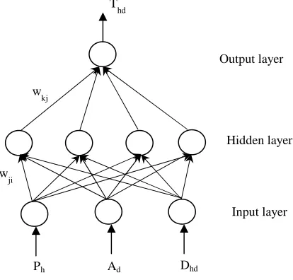
The structure of the ANN model is one of its key properties. The multilayer perceptron neural network is commonly used in many studies. This normally has three layers, namely input, output and hidden layers. Each layer has a number of nodes or processing units. Except for hidden layer nodes, the numbers of processing units are determined by the variables that construct the expected outputs. In the
case of work trip distribution-by analogy to the DCGM, the output Trip Flow (Thd) is a function of the inputs Trip
Production (Ph), Trip Attraction (Ad) and Trip Length (Cost)
(Dhd) (as the deterrence factor). Therefore, there are three
nodes at the input layer, while output layer has only one node (see Figure 1).
Fig. 1 Proposed neural network model structure
This study used a constant number of nodes in hidden layer as a recent study by Yaldi et al. [12] indicated that the number of nodes in that layer is not a significant factor in ANN model performance, as tested over a range of 0-20 nodes. Sometimes it would increase the error level, as found by Carvalho et al. [6]. Thus, in the present study the number of nodes in the hidden layer was set to be a constant number of ten nodes.
The training process is started from summation in the hidden layer nodes using the following general equation, for ANN node j receiving inputs from a set of nodes i.
(1)
where Oj is an output value, xi is an input signal, and wj-i
is a weighting value. Then, the Oj is compressed according
to the activation function used in the network structure, in this case Logsig. Thus, the transformed output in hidden layer nodes (O’j) is:
(2)
This is followed by the summation in the output layer node (Ok),
(3)
Since the same activation function is used in the output layer node, the summation result in this layer is squashed according to the following equation,
(4) Output layer
Hidden layer
Input layer w
kj
w
ji
Ph Ad Dhd
T
The result (estimated trip numbers/Thd) is then compared
with the target value (observed trip numbers, thd), and the
difference (diff) computed as follow,
(5)
The difference is then compared with the threshold value (goal). If it is below the threshold value, than the training is stopped, otherwise the error (diff) is backpropagated to the system in order to obtain the combination of connection weights that can generate results with error below the threshold value. This recursive process is undertaken using the procedure based on the Marquardt algorithm incorporated in the BP and termed as the Levenberg-Marquardt algorithm (LM) [10]. This algorithm was used due to its ability to converge faster [11, 13] and generate more accurate results.
The study used work trip data collected by the Transportation Agency of Padang City, West Sumatra, Indonesia. There are 36 traffic analysis zones covering the city, so that there are 1296 samples for all nodes in the input and output layers. The data are divided into training, validation and testing samples.
Data for training, validation and testing were randomly selected. The data were then divided to three parts, namely (1) 40% for training, (2) 30% for validation, and (3) 30% for testing. The input data values were normalized in the range [0, 1] according to the maximum value prior to the training. If x0 is an observed input value then the input data value xi is
given by xi = x0 / xmax where xmax is the maximum of the set
of observed values (x0) for the specific data set.
There are three scenarios used in this study as shown in Table 1. All properties for each scenario are the same, except the activation functions used in the output layer node. All nodes in the hidden layer use the Logsig activation function. The maximum epoch is limited to 100 iterations. The details of the scenarios are also reported in Table 1.
TABLEI
NEURAL NETWORK MODEL SCENARIO
#Scenario Data
normalization
Activation function #Exp Hidden
Layer
Output Layer
1 xi = xo/xmax Logsig Purelin 30 times
2 xi = xo/xmax Logsig Logsig 30 times
3 xi = xo/xmax Logsig Tansig 30 times
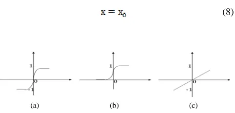
The activation functions will squash the summation output in both hidden and output layers according to the following formulae and Figure 2:
1. Tansig/double logistic (Figure 2a)
(6)
2. Logsig/logistic (Figure 2b)
(7)
3. Purelin
(8)
Fig. 2 Common activation functions used in NN
The model was developed using the Neural Network Tool in MATLAB. The initial weights for all layers were randomly selected by MATLAB. The weights were updated after all of the data were used in the training (batch mode). Model performance was measured using Root Mean Square Error (RMSE) and correlation coefficient (r). To enable the statistical tests, the experiments were run for 30 times for each scenario.
The tests and analysis were conducted at two levels, namely the calibration and testing/generalization performances. The comparison involves t-test for RMSE while χ2
and Fisher’s Z-transformation test for correlation coefficient (r).
III. RESULTS AND DISCUSSIONS
In order to illustrate the ability of ANN approach in estimating work trip distribution numbers, the experiment was conducted and evaluated at two levels, namely calibration and model testing (generalization). The DCGM calibrated by Hyman’s algorithm [14] is used to benchmark the ANN model performance (see Table 2 for DCGM calibration and testing performance details).
TABLEIII
DOUBLY CONSTRAINED GRAVITY MODEL PERFORMANCE
Deterrence function Exponential
Value of deterrence function parameter (ββββ) 0.11
RMSE-Calibration 168
RMSE-Generalization 174
Correlation coefficient-Calibration 0.82 Correlation coefficient-Testing 0.82
The details of the ANN calibration results for different activation functions are reported in Tables 3 and 4. The results for all scenarios suggest that the ANN approach can calibrate the work trip distribution with lower discrepancies between estimated and observed trip number (Thd – thd) than
the DCGM. The ANN models have significantly lower mean of RMSE than the DCGM as suggested by the t-test results (See Table 3).
The χ2 test suggests that the variations between each
experiment within the same scenario are insignificant suggesting training the ANN models by using Levenberg-Marquardt algorithm with random initial connection weights generates a statistically similar performance. The statistical test for the correlation coefficient (r) which is transformed to
the Fisher’s Z value indicates that ANN models can also distribute the trip numbers significantly closer to the original distribution pattern than the DCGM model calibrated using maximum likelihood. However, the testing results where the data is randomly split to 40, 30 and 30% for training, validation and testing suggest that the generalization performance of ANN model is still significantly lower than DCGM. The ANN models generate higher discrepancies (RMSE) and lower correlation coefficients (r) than DCGM (see Tables 5 and 6).
TABLEIII
RMSE FOR TRIPS (THD)(CALIBRATION)
Trial #
RMSE
Logsig-Tansig Logsig-Logsig Logsig-Purelin
1 160 159 157
2 164 153 161
3 160 159 157
4 161 159 157
5 153 154 159
6 163 155 159
7 160 160 161
8 157 159 160
9 159 159 156
10 162 158 159
11 162 158 163
12 156 149 161
13 152 155 162
14 161 160 159
15 163 153 161
16 160 167 156
17 164 155 161
18 159 154 159
19 161 160 160
20 159 149 159
21 159 167 162
22 162 158 160
23 166 154 158
24 162 159 162
25 158 157 155
26 159 148 161
27 162 152 159
28 161 164 161
29 158 155 159
30 161 156 159
Mean 160 157 159
t-test* -12.593 (2.045) -12.252 (2.045) -21.377 (2.045)
*Based on paired two-tailed t-test, degree of freedom is 29
The drawback in the ANN models presented in Tables 5 and 6 in terms of their testing performance may be influenced by two factors, namely (1) The activation function used in the models, and (2) The nature of the input data which is linearly normalized to its maximum value.
To estimate trip number distribution by using NN approach, an iterative procedure is conducted to minimize error (diff) between estimated and real trip numbers. The difference is computed as:
diff = Network Output – Observed Trip (9)
∆ = Thd – thd (10)
When Logsig or Tansig functions are used to transform the ANN model outputs in both hidden and output layers that means the results are nonlinearly normalized according to Figure 2a and 2b. Thus, the difference is computed as the gap between the nonlinearly transformed trip numbers (Thd)
and real trip numbers (thd), which is then linearly normalized
to restore its value range. Thus the difference becomes the gap between nonlinear model output and the linear data input, or:
∆ = (Non-Linear) Thd – (Linear) thd (11)
→ unmatched (Systematic error)!
The deviation between model output and observed trip numbers is obtained by comparing Figure 2a and 2c, or Figure 2b and 2c. This is incorrect as the comparison should be based on the same nature, nonlinear output data against nonlinear input data.
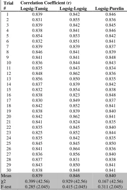
TABLEIV
CORRELATION COEFFICIENTS (R) FOR TRIPS (THD)(CALIBRATION)
Trial #
Correlation Coefficient (r)
Logsig-Tansig Logsig-Logsig Logsig-Purelin
1 0.839 0.842 0.846
2 0.831 0.855 0.836
3 0.839 0.842 0.845
4 0.838 0.841 0.846
5 0.854 0.853 0.842
6 0.832 0.851 0.841
7 0.839 0.839 0.837
8 0.846 0.841 0.839
9 0.841 0.841 0.848
10 0.836 0.844 0.843
11 0.835 0.843 0.834
12 0.848 0.862 0.836
13 0.856 0.850 0.835
14 0.837 0.839 0.842
15 0.832 0.854 0.838
16 0.838 0.823 0.848
17 0.830 0.849 0.837
18 0.842 0.852 0.841
19 0.838 0.839 0.840
20 0.842 0.862 0.841
21 0.841 0.824 0.835
22 0.835 0.845 0.840
23 0.825 0.852 0.844
24 0.835 0.842 0.835
25 0.845 0.845 0.850
26 0.841 0.864 0.836
27 0.836 0.856 0.840
28 0.837 0.831 0.838
29 0.843 0.850 0.841
30 0.838 0.848 0.841
Mean 0.839 0.846 0.840
TABLEV
RMSE FOR TRIPS (THD)(TESTING)
Trial #
RMSE
Logsig-Tansig Logsig-Logsig Logsig-Purelin
1 171 184 175
2 204 183 174
3 172 176 177
4 175 176 194
5 173 178 182
6 181 180 177
7 193 179 183
8 172 176 175
9 174 169 177
10 179 173 174
11 182 188 172
12 177 174 179
13 179 190 190
14 177 182 258
15 174 180 186
16 237 180 179
17 186 176 199
18 183 178 192
19 212 181 184
20 179 179 231
21 172 176 185
22 187 176 183
23 176 176 180
24 180 178 174
25 175 226 202
26 178 172 174
27 176 177 201
28 174 168 178
29 175 172 172
30 179 172 179
Mean 182 179 186
t-test 3.171 (2.045) 3.050 (2.045) 3.758 (2.045)
Thus there is a systematic mismatch in the difference computation in the above equation. Therefore, it needs to be corrected so that:
Corrected diff= (Non-Linear) Thd - (Non-Linear) thd (12)
→matched!
This correction is expressed through the nonlinear transformation of the input data including the Trip Production (Ph), Attraction (Ad), Distance (Dhd), and
observed Trip numbers (thd). It can be made by using the
following steps:
1. Normalize the raw data by using the following formulae:
xi= xo/xmax (13)
2. Transform the normalized data to nonlinear numbers by using the following formulas:
xi’= (2/(1+exp(-2xi))-1 (14)
→if transformed nonlinearly to Tansig
xi’= 1/(1+exp(-xi)) (15)
→ if transformed nonlinearly to Logsig
Then, the difference becomes:
diff = Network Output – Observed Trip (16)
∆ = Thd – thd (17)
∆ = (Non-Linear) Thd – (Non-Linear) thd (18)
→matched!
TABLEVI
CORRELATION COEFFICIENTS (R) FOR TRIPS (THD)(TESTING)
Trial #
Correlation Coefficient (r)
Logsig-Tansig Logsig-Logsig Logsig-Purelin
1 0.819 0.786 0.809
2 0.772 0.796 0.811
3 0.829 0.805 0.806
4 0.809 0.807 0.758
5 0.816 0.800 0.793
6 0.794 0.801 0.804
7 0.762 0.798 0.804
8 0.814 0.816 0.807
9 0.813 0.821 0.804
10 0.809 0.812 0.813
11 0.802 0.789 0.824
12 0.803 0.821 0.801
13 0.808 0.771 0.788
14 0.806 0.793 0.634
15 0.811 0.795 0.809
16 0.651 0.797 0.800
17 0.780 0.807 0.777
18 0.789 0.800 0.782
19 0.723 0.792 0.808
20 0.801 0.804 0.689
21 0.816 0.811 0.793
22 0.790 0.816 0.808
23 0.816 0.807 0.802
24 0.807 0.802 0.817
25 0.823 0.653 0.781
26 0.817 0.818 0.811
27 0.805 0.804 0.750
28 0.811 0.833 0.810
29 0.812 0.817 0.818
30 0.805 0.815 0.799
Mean 0.797 0.800 0.790
χ2 5.124 (42.56) 3.853 (42.56) 6.215 (42.56) F-test -0.434 (2.045) -0.407 (2.045) -0.524 (2.045)
Then, the network can be trained, validated and tested based on the nonlinear transformed data. Before measuring the performance of the modified ANN models, return its outputs to the original form, according to the following steps:
1. Return the results to linear form
xio = -0.5ln ((2/( xi+1))-1) (19)
→ if transformed to Tansig
xio= -ln ((1/( xi+1))-1) (20)
→ if transformed to Logsig
2. Return the results of previous step to the actual values
3. Measure the ANN model generalization performance (RMSE and r) for estimated trip numbers (Thd)
The results of the modified ANN models are reported in Tables 7-11 and Figures 3-6. The results suggest that nonlinearly transformed data can improve the testing performance of the ANN models. For example is indicated by the performance comparison of average RMSE and correlation coefficient between the ANN model before and after modification as reported in Tables 7 & 8. It can be seen that the ANN model performance normalized with Sigmoid nonlinear transformation tends to generate significantly lower RMSE and better goodness-of-fit compared to before modification.
The modification results also demonstrate the RMSE is now statistically different and lower than the DCGM once transformed to Logsig (see Table 9). The variations between each experiment within the same scenario are still insignificant and it is even lower than before as suggested by the results of χ2 test. The difference between the correlation
coefficient of ANN models is now statistically insignificant compared to the DCGM as reported in Table 10.
TABLEVII
AVERAGE RMSE FOR TRIPS (THD)(TESTING-BEFORE AND AFTER
TRANSFORMATION)
RMSE
Logsig-Tansig Logsig-Logsig Logsig-Purelin
Before 182 179 186
After 174 172 182
t-test 0.56 (2.045) 0.70 (2.045) 0.15 (2.045)
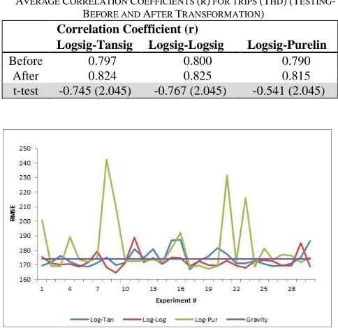
TABLEVIII
AVERAGE CORRELATION COEFFICIENTS (R) FOR TRIPS (THD)(TESTING -BEFORE AND AFTER TRANSFORMATION)
Correlation Coefficient (r)
Logsig-Tansig Logsig-Logsig Logsig-Purelin
Before 0.797 0.800 0.790
After 0.824 0.825 0.815
t-test -0.745 (2.045) -0.767 (2.045) -0.541 (2.045)
Fig. 3 NN Model testing performance/RMSE (Sigmoid nonlinear data transformation) compared with DCGM
TABLEIX
RMSE FOR TRIPS (THD)(TESTING-SIGMOID NONLINEAR DATA TRANSFORMATION)
Trial #
RMSE
Logsig-Tansig Logsig-Logsig Logsig-Purelin
1 169 175 201
2 172 171 169
3 176 170 169
4 172 171 189
5 169 169 174
6 169 172 172
7 171 179 175
8 175 168 242
9 170 165 210
10 172 171 172
11 181 189 172
12 175 172 173
13 181 175 174
14 171 171 172
15 187 175 182
16 187 175 192
17 167 169 169
18 173 172 169
19 176 170 167
20 182 169 169
21 178 173 231
22 171 170 172
23 171 168 216
24 173 172 169
25 171 173 181
26 169 173 174
27 169 169 177
28 171 169 176
29 175 185 172
30 187 169 175
Mean 174 172 182
t-test 0.613 (2.045) -1.536 (2.045) 2.334 (2.045)
Fig. 4 NN Model testing performance/Correlation Coefficient (r) (Sigmoid nonlinear data transformation) compared with DCGM
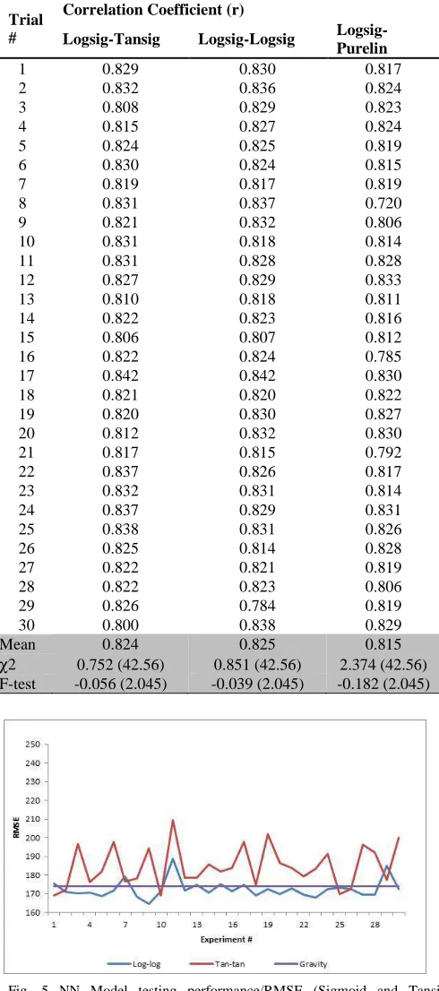
Although the Logsig-Purelin scenario performance is also improved, it is still below the DCGM. In addition, there is a significantly different RMSE and correlation coefficient between each experiment within this scenario (see also Figures 3 and 4). This is because the data in the ANN model outputs are not transformed to nonlinear form during the iteration process as it used linear transfer function (Purelin).
The RMSE and correlation coefficient are statistically the same as DCGM. However, this model has a higher RMSE and a lower correlation coefficient than DCGM and Logsig transformed data. Further, the performance fluctuation of the ANN models whithin this scenario is more obvious than the Logsig-logsig scenario (see Figures 5 and 6).
TABLEX
CORRELATION COEFFICIENTS (R) FOR TRIPS (THD)(TESTING-SIGMOID NONLINEAR DATA TRANSFORMATION)
Trial #
Correlation Coefficient (r)
Logsig-Tansig Logsig-Logsig Logsig-Purelin
1 0.829 0.830 0.817
2 0.832 0.836 0.824
3 0.808 0.829 0.823
4 0.815 0.827 0.824
5 0.824 0.825 0.819
6 0.830 0.824 0.815
7 0.819 0.817 0.819
8 0.831 0.837 0.720
9 0.821 0.832 0.806
10 0.831 0.818 0.814
11 0.831 0.828 0.828
12 0.827 0.829 0.833
13 0.810 0.818 0.811
14 0.822 0.823 0.816
15 0.806 0.807 0.812
16 0.822 0.824 0.785
17 0.842 0.842 0.830
18 0.821 0.820 0.822
19 0.820 0.830 0.827
20 0.812 0.832 0.830
21 0.817 0.815 0.792
22 0.837 0.826 0.817
23 0.832 0.831 0.814
24 0.837 0.829 0.831
25 0.838 0.831 0.826
26 0.825 0.814 0.828
27 0.822 0.821 0.819
28 0.822 0.823 0.806
29 0.826 0.784 0.819
30 0.800 0.838 0.829
Mean 0.824 0.825 0.815
χ2 0.752 (42.56) 0.851 (42.56) 2.374 (42.56) F-test -0.056 (2.045) -0.039 (2.045) -0.182 (2.045)
Fig. 5 NN Model testing performance/RMSE (Sigmoid and Tansig nonlinear data transformation) compared with DCGM
Fig. 6 NN Model testing performance/Correlation Coefficient (r) (Sigmoid and Tansig nonlinear data transformation) compared with DCGM
TABLEXI
RMSE AND CORRELATION COEFFICIENTS (R) FOR TRIPS (TIJ) (NONLINEAR TRANSFORMATION-LOGSIG &TANSIG)
Trial #
RMSE Correlation Coefficient (r)
Logsig-Tansig
Logsig
-Logsig Logsig-Tansig Logsig-Logsig
1 169 175 0.825 0.830
2 172 171 0.817 0.836
3 197 170 0.776 0.829
4 176 171 0.817 0.827
5 182 169 0.793 0.825
6 198 172 0.773 0.824
7 177 179 0.805 0.817
8 178 168 0.816 0.837
9 195 165 0.780 0.832
10 169 171 0.826 0.818
11 209 189 0.781 0.828
12 178 172 0.817 0.829
13 179 175 0.815 0.818
14 186 171 0.785 0.823
15 182 175 0.815 0.807
16 184 171 0.791 0.817
17 198 175 0.762 0.824
18 175 169 0.821 0.842
19 202 172 0.767 0.820
20 187 170 0.789 0.830
21 184 173 0.800 0.815
22 179 170 0.820 0.826
23 183 168 0.803 0.831
24 191 172 0.779 0.829
25 170 173 0.831 0.831
26 173 173 0.830 0.814
27 196 169 0.771 0.821
28 192 169 0.783 0.823
29 177 185 0.815 0.784
30 200 173 0.761 0.813
Mean 185 172 0.799 0.823
t-test 5.534 (2.045)
-1.336 (2.045)
χ2 2.877 (42.56) 0.823 (42.56)
F-test -0.023 (2.045) -0.061 (2.045)
IV. CONCLUSIONS
approach. The testing results suggest that the ANN models can significantly outperform the equivalent gravity models, after the input data is transformed by logistic function. Hence, nonlinearly transformed data can improve the testing performance of the ANN model.
The Logistic transfer function is found to be the most appropriate transformation function in both hidden and output layers for work trip number distribution. Finally, the ANN models can be used as a potential alternative method in calibrating and estimating the work trip number distribution with a higher accuracy than the well-established technique of the doubly constrained gravity model.
NOMENCLATURE
A Trip Attraction Trip
D Deterrence factor Km
diff Difference
Exp Exponential
ln Natural logarithm
o ANN Output value
P Trip Production Trip
r Correlation coefficient
RMSE Root Mean Square Error Trip
t Observed trip number Trip
T Estimated trip number Trip
x ANN input signal
w Connection weight
Greek letters
∆ Delta Trip
′ squashed summation value
χ2 Chi square
Subscripts
d zone d
0 original value
h zone h
i input layer
j hidden layer
k output layer
max maximum value
REFERENCES
[1] W. R. Black, "Spatial interaction modeling using artificial neural networks," Journal of Transport Geography, vol. 3, pp. 159-166, 1995.
[2] M. Tanaka and N. Uno, "Evaluation of Car-Following Input Variables and Development of Three-Vehicle Car-Following Models with Artificial Neural Networks," Journal of the Eastern Asia Society for Transportation Studies, vol. 11, pp. 1826-1841, 2015.
[3] M. Dougherty, "A review of neural networks applied to transport," Transportation Research Part C: Emerging Technologies, vol. 3, pp. 247-260, 1995.
[4] M. Mozolin, et al., "Trip distribution forecasting with multilayer perceptron neural networks: A critical evaluation," Transportation Research Part B: Methodological, vol. 34, pp. 53-73, 2000. [5] D. Teodorovic and K. Vukadinovic, Traffic Control and Transport
Planning: A Fuzzy Sets and Neural Networks Approach. Massachusetts, USA: Kluwer Academic Publisher, 1998.
[6] M. C. M. Carvalho, et al., "Forecasting travel demand: a comparison of logit and artificial neural network methods," The Journal of the Operational Research Society, vol. 49, pp. 711-722, 1998.
[7] Yaldi, G., Taylor, M. A. P. & Yue, W. L., "Improving Artificial Neural Network Performance in Calibrating Doubly-Constrained Work Trip Distribution by Using a Simple Data Normalization and Linear Activation Function," in Paper of The 32 Australasian Transportation Research Forum, Auckland, New Zealand. Available at www.patrec.org/atrf.aspx, 2009.
[8] Yaldi, G., Taylor, M. A. P. & Yue, W. L., "Forecasting origin-destination matrices by using neural network approach: A comparison of testing performance between back propagation, variable learning rate and levenberg-marquardt algorithms," in Australasian Transport Research Forum, Adelaide, Australia, 2011. [9] D. W. Marquardt, "An Algorithm for Least-Squares Estimation of
Nonlinear Parameters," Journal of the Society for Industrial and Applied Mathematics, vol. 11, pp. 431-441, 1963.
[10] M. T. Hagan and M. B. Menhaj, "Training feedforward networks with the Marquardt algorithm," IEEE Transactions on Neural Networks vol. 5, pp. 989-993, 1994.
[11] G. Yaldi, "A Deeper Insight of Neural Network Spatial Interaction Model's Performance Trained with Different Training Algorithms," Journal of the Eastern Asia Society for Transportation Studies, vol. 11, pp. 342-361, 2015.
[12] G. Yaldi, "Analysing the Behaviour and Performance of Neural Network Trip Distribution Models toward Different Hidden Layer and Node Numbers," presented at the The 11th International Conference of Eastern Asia Society for Transportation Studies, Cebu, Philippines, 2015.
[13] J. Amita, et al., "Prediction of Bus Travel Time using ANN: A Case Study in Delhi," Transportation Research Procedia, vol. 17, pp. 263 – 272, 2016.