Vol.8 (2018) No. 4-2
ISSN: 2088-5334
Cosine Harmony Search (CHS) for Static Optimization
Farah Aqilah Bohani
#, Siti Norul Huda Sheikh Abdullah
#, Khairuddin Omar
##
Faculty of Information Science and Technology,
The National University of Malaysia, 43600, Bangi, Selangor, Malaysia E-mail: [email protected], [email protected], [email protected]
Abstract— Harmony Search (HS) is the behaviour imitation of a musician looking for a balanced harmony. HS has difficulty finding
the best tuning parameter, especially for Pitch Adjustment Rate (PAR). PAR plays a crucial role in selecting historical solution and adjusting it using Bandwidth (BW) value. PAR in HS requires a constant value to be initialized. Furthermore, there is a delay in convergence speed due to the disproportion of global and local search capabilities. Although some HS variants have claimed to overcome this shortcoming by introducing the self-modification of PAR, these justifications have been found to be imprecise and require more extensive experiments. Local Opposition-Based Learning Self-Adaptation Global Harmony Search (LHS) implements a heuristic factor, η for self-modification of PAR. It (η) manages the probability for selecting the adaptive step, either global adaptive step or worst adaptive step. If the value of η is large, the prospects of selecting the global adaptive step is higher, thereby allowing the algorithm to exploit a better harmony value. Conversely, if η is small, the worst adaptive step is prone to selection, therefore the algorithm is closed to the best global solution. In this paper, in addressing the existing HS obstacle, we introduce a Cosine Harmony Search (CHS) which incorporates an additional strategy rule. This additional strategy employs the η inspired by LHS and contains the cosine parameter. This allows for self-modification of pitch tuning to enlarge the exploitation capabilities. We test our proposed CHS on twelve standard static benchmark functions and compare it with basic HS and five state-of-the-art HS variants. Our proposed method and these state-of-the-art algorithms are executed using 30 and 50 dimensions. The numerical results demonstrated that the CHS has outperformed other state-of-the-art algorithms in terms of accuracy and convergence speed evaluations.
Keywords— additional strategy rule; cosine; global pitch adjustment; accuracy; convergence speed.
I. INTRODUCTION
Harmony Search (HS) was introduced by Geem in 2001 [1] which imitates the behavior of a musician looking for a well-balanced harmony. HS has the advantages of having a simple model and good performance in the global search domain. Furthermore, HS has been employed and engaged in numerous real-world optimization problems [2-10]. Research in HS is still striving to introduce a mechanism to find the best tuning parameters, especially the Pitch Adjustment Rate (PAR). PAR plays a crucial role in selecting historical solution and adjusting it using Bandwidth (BW) value [11]. Currently, PAR in HS needs to be initialized with a constant value at the initial step. This effects the convergence time due to a disproportion of global and local search capabilities [12]. Consequently, HS falls easily into the local optimum and produces low accuracy [13].
Other than PAR, Harmony Memory Consideration Rate (HMCR) is another element that can be utilized to select historical solution. HCMR frequently uses BW for parameter tuning. Therefore, both HCMR and PAR play an important
role in HS for the exploitation process. Exploitation refers to a better global solution relying on a better local solution. This study aims to improve the exploitation capability of HS. Many variants of HS have been proposed to overcome this problem, namely Improved Harmony Search (IHS) [13], Improved Global-Best Harmony Search Algorithm (IGHS) [14], Global-Best Harmony Search (GHS) [15], Self-Adaptive Harmony Search Algorithm (SAHS) [16], Cooperative-Competitive Master-Slave Multi-Population GHS (CC-GHS) [17], Enhance Basic HSA (called EHSA) [18], Meta-HSA [19], Dual Population Multi Operators Harmony Search Algorithm [20], and A Multi-Population Harmony Search Algorithm [21]. However, these HS variants are still poor in terms of performance, in particular, the accuracy and robustness in solving numerical optimization problems. Hence, Local Opposition-Based Learning Self-Adaptation Global Harmony Search (LHS) has been proposed [11] to overcome this issue. LHS become more effective through the introduction of self-modification of pitch tuning at first key improvements whereby its exploitation ability of solution space increased [11].
generate self-modification of pitch tuning in LHS. It determines value in three steps, involving early, middle and late stages. Although LHS has higher local exploitation capabilities with the self-modification of pitch tuning, its restraint into three stages may limit its global exploitation capabilities. Thus, this paper proposes a new rule for determining value by embedding a cosine parameter. This improvisation of the self-modification of pitch tuning is called Cosine Harmony Search (CHS). This addition that now results in four stages, further expands the exploitation capabilities. As a result, CHS is able to exploit more search space and provides better results than current state-of-the-art algorithms. This approach will eventually serve as an alternative solution to the static optimization problems.
In line with the objectives of this research, this study was conducted on twelve standard static benchmark functions for optimization tests to verify our proposed idea. We also compared CHS with existing state-of-the-art approaches, namely basic HS, IHS, GHS, IGHS, SAHS and LHS, across two dimensions comprising of 30 and 50 variables which have been widely used in static optimization studies.
The rest of the paper is arranged as follows: Section 2 indicates material and method of this paper; Section 3 presents results and discussion; Section 4 concludes with a summary of the findings and possible future work.
II. MATERIAL AND METHOD
A. Related Material
The basic HS algorithm is a stochastic global optimizer and population-based. Five steps of HS searching are; (1). Initialize the optimization problem and algorithm parameter such as maximum size of harmony memory (HMS), pitch adjusting rate (PAR), harmony memory consideration rate (HMCR), Bandwidth (BW), maximal iteration number ( ) and current iteration , (2). Initialize the harmony memory, (3). Improvise a new harmony from harmony memory (HM), (4). Update harmony memory and (5). Test the termination condition [1]. It also requires three parameters: HMS, HMCR and PAR with a constant value at the first step.
Importantly, a new harmony generated by HS is relying on PAR. Generally, PAR plays an important role in the exploitation mechanism in HS. PAR with constant value at the first step may affect the exploitation capabilities of HS, hence making it harder to yield better global solutions.
Initially, if random number 1 is smaller than HMCR, then it employs the consideration of harmony memory,
, = , . This equation considers as one of the
elements, ranged from 1 to , such as ∈ 1,2,3, … , . In this case, denotes the maximal dimensions. ∈
1,2,3, … , denotes the harmony index.
Subsequently, if 2 represents a random number less than PAR value, then fine-tune decision variables , , such as in Eq.(1),
, =
⎩ ⎨
⎧ if , + $ × &',
*≤ ,-. /≤ 0.5 .
, − $ × &',
if *≤ ,-. /> 0.5.
(1)
where $ is a number in the range [-1, 1] which is consistently divided in random. The parameter of &' is remains as a solid value.
If 1 is greater than HMCR, then a new harmony provided, as seen in Eq.(2),
, = ,4+ × ( ,5− ,4), (2)
where is a number in the range [0, 1] and is homogenously distributed at random.
A different harmony is generated through cycles, on which the fitness is then computed. Next, check the condition of fitness of harmony memory. For example, if new harmony is better than worst harmony, choose new harmony as a better harmony, otherwise choose worst harmony.
Finally, the criteria for the termination condition is analysed. If , the number of maximal iterations is fulfilled, then the computation is discontinued. Contrarily, all of the processes will rerun.
B. Improved Harmony Search (LHS)
LHS has advantage in self-modification of pitch tuning due to enhance the exploitative ability. LHS applies the two harmonies which are the best harmony and the worst harmony regarding to achieve an optimal solution [11].
The self-modification of pitch tuning in LHS indicates that the heuristic factor, is introduced to enable dynamical increment with the generation number. The self-modification of pitch tuning shown in Eq.(3).
,
= 6 , , + × 7 8 9:, − , ; , if ≤
, , − × 7 < 9:, − , ;, otherwise,
(3)
where is a new candidate harmony vector, , is the
jth components of . < 9:, denotes the jth components of the worst harmony in HM, whereas 8 9:, denotes the th component of the best harmony. is a heuristic factor, which characterizes the searching process. The parameter manages the probability of selecting the adaptive step – either global or worst.
The expression wherein and are the maximal and current iteration numbers respectively, are shown in Eq.(4). The completed LHS algorithm is shown in Algorithm 1. ,-.DE and ,-.DFG in Algorithm 1 are the minimum and
maximum adjusting rates respectively. In addition, is the maximum number of iterations, whereas represents the current iteration.
=
⎩ ⎪ ⎨ ⎪
⎧ I1 − (1.5 ), < /2
0.5, /2 ≤ < 3 /4
exp (−(O14.53 − 14.04 / )), otherwise. (4)
Algorithm 1: LHS [11]
Input: Maximum size of harmony memory , maximal dimension , maximal generation P, ,-.DE and ,-.DFG.
Output :worst harmony, < 9: , function objective of worst harmony Q( < 9:)
Step 1:Initialize parameters of harmony search such as HMS, D,G, ,-.DE and ,-.DFG.
Step 2: Initialize harmony memory as below: For i=1 to HMS do
For j=1 to D
E, = ,4+ . ( ,5− ,4);
End For Calculate Q( E )
End For
Step 3: Improvise g=0, while the termination criteria is inadequate (g<G) do
For j=1 to D do If rand()≤HMCR
% memory consideration
, R ,( ∈ 1,2,3, … );
S , = ,5+ ,4− ,;
Calculate the parameter η such as Eq.(4) % pitch adjustment
Execute Eq.(3) End If Else
% random selection
, = ,4+ . ( ,5− ,4) ; S , = ,4+ . ( ,5− ,4) ; End If
End For
Step 4: Update the worst harmony
Select the worst harmony vector < 9: in the current harmony memory and calculate Q( ) and Q(S_ UV)
If Q( ) < Q(S )
< 9:= ;
Q( < 9:) = Q( );
Else
< 9:= S ;
Q( < 9:) = Q(S );
End If W = W + 1 ; End While
Step 5: Algorithm stops after obtaining the best solution is obtained
C. Our Proposed Method: Cosine Harmony Search (CHS)
Cosine Harmony Search (CHS) has been inspired by LHS, and has three similar key features [11]; 1. self-modification of pitch tuning; 2. opposition-based learning technique; and 3. competition selection mechanism. These features are shown in Algorithm 2.
CHS has four stages to determine the value of η. The operation of the third stage in CHS is based on the second stage in LHS, while the operation of the fourth stage in CHS is similar to the third stage of LHS. The modification to a four-stage system occurs in the first and second stages of CHS. The first and second stages in CHS have been embedded with a cosine parameter. The part of the first stage,
which is k<Z
[ , has embedded cosine parameter multiplied
by parameter α]. Then, the part of the second stage which is
Z [< k <
Z
* has embedded cosine parameter multiplied by
parameter α*. The proposed additional strategy rule to determine the value of η is shown in Eq.(5). This parameter is designed to increase exploitation while avoiding being trapped in the local optima.
Algorithm 2: The proposed CHS
Input: Maximum size of harmony memory , maximal dimension , maximal generation P, ,-.DE and ,-.DFG.
Output :worst harmony, < 9: , function objective of worst harmony Q( < 9:)
Step 1:I Initialize parameters of harmony search such as HMS, D,G, ,-.DE and ,-.DFG.
Step 2: Initialize harmony memory as below: For i=1 to HMS do
For j=1 to
E, = ,4+ . ( ,5− ,4);
End For Calculate Q( E )
End For
Step 3: Improvise g=0, while the termination criteria is inadequate (g<G) do
For j=1 to do If rand()≤HMCR
% memory consideration
, R ,( ∈ 1,2,3, … );
S , = ,5+ ,4− ,;
Calculate the parameter η such as Eq.(5) % pitch adjustment
Execute Eq.(3) End If Else
% random selection , = ,4+ . ( ,5− ,4) ;
S , = ,4+ . ( ,5− ,4) ;
End If End For
Step 4: Update the worst harmony
Select the worst harmony vector < 9: in the current harmony memory and calculate Q( ) and Q(S_ UV)
If Q( ) < Q(S )
< 9:= ;
Q( < 9:) = Q( );
Else
< 9:= S ;
Q( < 9:) = Q(S );
End If
W End While
Step 5: Algorithm stops after the best solution is obtained
= ⎩ ⎪ ⎪ ⎪ ⎪ ⎪ ⎨ ⎪ ⎪ ⎪ ⎪ ⎪
⎧ I1 −^1.5 _× cos(a)×b] , < 4 ,
I1 − ^1.5 _ × cos(a) × b* , 4 < < 2 ,
0.5, 2 ≤ <34 ,
exp c− dI14.53 −14.04 ef , others,
where cos(a) = cos(45),b]= 1.8 and b*= 2.4 .
D. Experimental Setup
Other HS variants and the proposed CHS algorithms has compared and analyzed by using the 12 standard static benchmark functions implemented in the Matlab Language with Intel (R) Core ™ i7-2620M CPU @ 2.70GHz 2.70 GHz and 4.00 GB RAM under operation system Microsoft 10 Pro. The functions have been used not only for the HS algorithm, but also for other metaheuristic algorithms [22, 23] . Table 1 shows the list of the 12 test functions including the characteristics, initial rate and global optimal value. All of the parameters for the proposed method and other algorithms were set according to Table II. For two set dimensions ,
which are 30 and 50, they represent the scalability of the algorithms in terms of their optimization performance. The maximum number of evaluations for the proposed method is set to 3000. Each of the evaluations is accomplished 50 times independently.
III.RESULTS AND DISCUSSION
The results are organized as follows: Subsection A shows the mean value from objective functions derived from each algorithm using 30 dimensions. Subsection B presents the mean value of objective functions conducted from each algorithm using 50 dimensions. The near global optimal solutions are also highlighted after being tested on 12 test functions. Subsection C explains the success rate (SR) for our proposed method (CHS) and HS variant after testing on both dimensions - 30D and 50D.
A. Proposed Method (CHS) and HS variant for 30D
Table III and Table IV illustrate the objectives of the value function for the optimization of the problem hi− hij for the proposed method, CHS and competing algorithms such as IHS, GHS, SAHS, IGHS, LHS and HS with 30 and 50 dimensions, respectively.
Table III shows that the proposed CHS has better optima solution than GHS, SAHS and basic HS in all test functions. CHS successfully yields better optimal solution than LHS in test function hk which is multimodal separable optimization problem.
The self-modification of pitch tuning mechanism with the embedment of a cosine parameter through a new rule construction of parameter determination present in CHS was able to improve its performance of the algorithm.
CHS finds the same optimum solution with IGHS and LHS in two test functions which are hl and hm. IHS is subpar in this context because it depends on possible value of parameter BW and PAR. The parameter dynamically changes with iteration numbers that caused IHS is hardly served in the global search.
In another case, GHS converges prematurely, whereby it has not assumed that the current best harmony may yield an optimal solution for local search.
B. Proposed Method (CHS) and HS variant for 50D
To evaluate the scalability of CHS, test functions hi− hij increased its dimension up to 50 dimensions. The maximum iteration is 3000, with 50 run independently.
Based on Table IV, CHS surpasses in test function hk compared to other algorithms, and has better optimal solutions than when run in 30 dimensions.
In the case of dimension increment up to 50 dimensions, CHS still produces equally optimal solutions, where 0 value on hl and hm are similar to test functions with 30 dimensions.
CHS has shown better results in hiiwith 30 dimensions than 50 dimensions.
SAHS proposed a new operation of pitch adjusting, providing better results with 50 dimensions compared to 30 dimensions on test function hl. Unfortunately, IHS and GHS
are less efficient in comparison to the state-of-the-art algorithms even when the dimension is increased.
Even though LHS outperforms others algorithm on all of test functions, CHS successfully achieves a near-same global optimal solution with LHS on 6 test functions, hn− ho and hm− hii in 30 dimensions. In 50 dimensions, CHS successfully achieves a near-same global optimas solution with LHS on 5 test function, hn− ho and hm− hip . This
proves that CHS is comparable.
In comparing basic HS with other algorithms in 30 and 50 dimensions on all test functions, basic HS performs poorly. Basic HS yields better results in 30 dimensions than in 50 dimensions.
C. Success Rate (SR) for Proposed Method (CHS) and HS variant with 30D and 50D
To compare the reliability of CHS with other HS variants for optimization problemshi− hij , the success rate (SR) is
considered. Table V and Table VI shows SR of CHS and other HS variants for 30 and 50 dimensions respectively.
CHS ranks third in SR average in 30 dimensions with 75%, followed by IHS, GHS, SAHS and basic HS, with an SR average of 23%, 16%, 11% and 0% respectively. LHS leads with 92%, followed by IGHS.
In 50 dimensions, the SR average of IHS, GHS, SAHS, IGHS and LHS are unreported in literature. In comparing CHS with basic HS, CHS outperforms basic HS with 73.83%. CHS achieved better SR average in 30 dimensions than 50 dimensions. Based on achievement of CHS in terms of SR average in 30 and 50 dimension, CHS is considered as comparable.
D. Convergence of Our Proposed Method (CHS)
To further analyze the convergence of the CHS, we used four test functions to compare the proposed method with basic HS. The first test was a Sphere function (qi), the second was a Rosenbrock function (qn), the third test was a Rastrigin function (qm), and the fourth test was an Ackley function (qip) with unimodal separable, unimodal separable, multimodal separable and multimodal non-separable tests respectively. These functions were tested on 30 dimensions.
TABLEI
STANDARDSTATICBENCHMARKFUNCTIONS(FN:FUNCTION NAME,FM:FUNCTION MODEL,C:CHARACTERISTIC,IR:INITIAL RANGE,GOV: GLOBAL OPTIMUM VALUE
FN FM C IR GOV
Sphere
Q]= r ]² t
ER]
US u−100,100vt 0
Schwefel 2.22
Q*= r‖ E‖ + x‖ E‖ t
ER] t
ER]
UN u−100,100vt 0
Schwefel 1.2
Q/= r dr E
R]
e²
t
ER]
UN u−100,100vt 0
Schwefel 2.21
Q[= max | E|, 1 ≤ | ≤
US u−100,100vt 0
Rosenbrock
Q}= ru100( E~]− E)*+ ( E− 1)²v
t•]
ER]
UN u−30,30vt 0
Step
Q€= r(⌊ E+ 0.5⌋) t
ER]
²
US u−100,100vt 0
Quartic
Qƒ= r | E[+ randomu0,1v t
ER]
US u−1.28,1.28vt 0
Schwefel
Q†= r − E× ‡| t
ER]
O‖ E‖
MS u−500,500vt -418.9829D
Rastrigin
Qˆ= ru E*− 10‰Š‡ t
ER]
(2‹ E) + 10v
MS u−5.12,5.12vt 0
Ackley
Q]Œ= −20 exp
⎝
⎛−0.2•1 r E* t
ER] ⎠
⎞ − exp’1 r cos2‹ E t
ER]
“ + 20U
MN u−32,32vt 0
Griewank
Q]]=4000 ’r1 E* t
ER]
“ − x ‰Š‡ ^ E
√| • _
t
ER]
+ 1
MN u−600,600vt 0
Penalized
Q]*=‹ 10 sin*(π—E) + r(—E− 1) * t
ER]
u1 + 10sin*(‹— E~])v
+(— − 1) * + r u(
E, 10,100,4)—E t
ER]
= 1 + 14 ( E+ 1)
TABLEII
PARAMETER SETTING OF PROPOSED METHOD (CHS)AND OTHER HSVARIANT (SIGN [-]REPRESENTS NOT RELATED)
Parameter Algorithms
HS IHS GHS SAHS IGHS LHS CHS
™. 0.99 0.9 0.9 0.9 0.99 0.99 0.99
5 5 5 5 5 5 5
,-.DE 0.1 0.1 0.1 0 0.01 - -
,-.DFG - 0.99 0.99 1 0.99 - -
,-. 0.1 - - - -
šVDE - 0.0001 - - 0.0001 - -
šVDFG - ( 5− 4)/ 20 - - ( 5− 4)/ 20 - -
šV 0.1 - - - -
b] - - - 1.8
b* - - - 2.4
cos - - - a =45
TABLEIII
MEAN OF OBJECTIVE FUNCTION AND STANDARD DEVIATION FOR PROBLEMS hi− hij( = 30) BY CHS AND OTHER HSVARIANT
IHS GHS SAHS IGHS LHS HS CHS
Mean Standard
deviation Mean
Standard deviation Mean
Standard deviation Mean
Standard
deviation Mean
Standard
deviation Mean
Standard
deviation Mean
Standard deviation
f1 5.38E-07 1.45E-07 1.07E+01 4.62E+00 1.35E+00 7.31E-01 0.00E+00 0.00E+00 0.00E+00 0.00E+00 2.74E+01 1.92E+01 2.10E-247 0.00E+00
f2 1.55E-01 4.09E-01 1.06E+01 2.07E+00 3.28E+00 7.89E-01 0.00E+00 0.00E+00 5.51E-260 0.00E+00 1.60E+01 4.65E+00 7.45E-142 5.03E-141
f3 4.17E+03 1.11E+03 4.47E+03 1.33E+03 8.73E+03 2.76E+03 1.42E-30 7.72E-30 7.73E-66 4.18E-65 2.08E+04 4.92E+03 1.70E-39 1.18E-38
f4 6.70E+00 9.80E-01 7.03E+00 8.92E-01 6.35E+00 1.26E+00 1.47E-132 7.13E-132 1.30E-143 7.04E-143 1.83E+01 4.16E+00 1.44E-89 6.16E-89
f5 1.77E+02 1.34E+02 5.06E+02 3.12E+02 3.69E+02 1.70E+02 2.78E+01 8.56E-01 2.68E+01 5.76E-01 3.82E+02 4.63E+02 3.14E+01 1.67E+01
f6 1.63E+00 1.50E+00 1.21E+01 3.96E+00 2.47E+00 1.57E+00 0.00E+00 0.00E+00 0.00E+00 0.00E+00 5.07E+01 1.71E+01 0.00E+00 0.00E+00
f7 6.46E-02 1.88E-02 8.60E-02 3.71E-02 7.80E-02 2.79E-02 5.69E-04 2.58E-04 2.83E-04 1.82E-04 2.27E-01 6.58E-02 6.76E-04 6.21E-04
f8 -1.26E+04 4.52E-01 -1.25E+04 9.74E+00 -1.26E+04 3.24E+00 -7.54E+03 4.74E+02 -1.26E+04 2.25E-06 1.26E+02 5.13E+01 -8.28E+30 5.82E+31
f9 2.14E+00 1.28E+00 3.83E+00 1.11E+00 1.11E+00 5.63E-01 0.00E+00 0.00E+00 0.00E+00 0.00E+00 4.76E+00 1.72E+00 0.00E+00 0.00E+00
f10 3.01E-01 3.47E-01 1.64E+00 3.01E-01 4.80E-01 1.92E-01 4.74E-15 1.70E-15 3.08E-15 1.23E-15 2.38E+00 3.53E-01 4.37E-15 5.02E-16
f11 2.27E-02 6.04E-02 1.10E+00 3.34E-02 7.83E-01 1.82E-01 9.04E-04 2.86E-03 0.00E+00 0.00E+00 1.41E+00 1.38E-01 0.00E+00 0.00E+00
f12 2.28E-02 2.96E-02 5.38E-02 5.36E-02 1.69E-02 2.86E-02 9.99E-02 9.80E-02 4.43E-08 8.66E-08 2.88E-01 1.72E-01 3.08E-02 1.92E-02
TABLEIV
MEAN OF OBJECTIVE FUNCTION AND STANDARD DEVIATION FOR PROBLEMS hi− hij( = 50) BY CHS AND OTHER HSVARIANT
IHS GHS SAHS IGHS LHS HS CHS
Mean Standard
deviation Mean
Standard deviation Mean
Standard deviation Mean
Standard
deviation Mean
Standard
deviation Mean
Standard
deviation Mean
Standard deviation
f1 2.70E+01 1.02E+01 5.38E+01 1.54E+01 2.18E-01 1.25E-01 7.83E-07 6.94E-08 0.00E+00 0.00E+00 8.63E+01 3.30E+01 6.74E-172 0.00E+00
f2 1.44E+01 3.77E+00 2.84E+01 3.63E+00 1.66E+00 4.14E-01 3.67E-02 1.74E-01 0.00E+00 0.00E+00 4.84E+04 1.03E+04 2.87E-97 1.59E-96
f3 1.31E+04 2.60E+03 1.30E+04 2.85E+03 1.10E+04 2.52E+03 1.85E-01 7.42E-02 4.03E-279 0.00E+00 4.95E+04 8.67E+03 6.13E-03 4.21E-02
f4 1.11E+01 1.12E+00 1.15E+01 1.06E+00 3.51E+00 5.05E-01 4.49E-04 3.25E-05 0.00E+00 0.00E+00 2.97E+01 4.37E+00 3.10E-64 1.08E-63
f5 1.17E+03 6.92E+02 1.59E+03 6.97E+02 1.78E+02 4.42E+01 6.12E+01 3.23E+01 4.58E+01 1.78E-01 1.53E+03 7.06E+02 5.41E+01 2.23E+01
f6 3.91E+01 1.39E+01 6.04E+01 1.90E+01 0.00E+00 0.00E+00 3.33E-02 1.83E-01 0.00E+00 0.00E+00 1.17E+02 3.37E+01 0.00E+00 0.00E+00
f7 1.46E-01 3.45E-02 2.06E-01 6.19E-02 5.88E-02 1.87E-02 7.42E-03 1.94E-03 6.73E-05 3.94E-05 4.25E-01 1.12E-01 9.56E-04 6.17E-04
f8 -2.09E+04 2.48E+01 -2.08E+04 4.61E+01 -2.09E+04 4.31E-01 -2.09E+04 9.56E-09 -2.09E+04 1.08E-05 2.91E+02 7.49E+01 -7.14E+29 3.50E+30
f9 1.24E+01 2.32E+00 1.58E+01 2.32E+00 1.36E-01 5.60E-02 1.46E-04 1.61E-05 0.00E+00 0.00E+00 1.04E+01 3.14E+00 0.00E+00 0.00E+00
f10 2.13E+00 3.13E-01 2.76E+00 2.86E-01 1.11E-01 3.68E-02 4.97E-04 1.77E-05 3.43E-15 6.49E-16 2.72E+00 2.53E-01 4.37E-15 5.02E-16
TABLEV
SUCCESS RATE (%)ACHIEVED BY PROBLEMShi− hij ( = 30) BY CHS AND OTHER HSVARIANT
IHS GHS SAHS IGHS LHS HS CHS
f1 0 0 0 100 100 0 100
f2 0 0 0 100 100 0 100
f3 0 0 0 100 100 0 100
f4 0 0 0 90 100 0 100
f5 2.5 0 0 0 0 0 0
f6 100 100 100 100 100 0 100
f7 0 0 0 75 100 0 0
f8 65 60 15 30 100 0 100
f9 0 0 0 100 100 0 100
f10 0 0 0 100 100 0 100
f11 0 0 0 100 100 0 100
f12 100 27.5 12.5 100 100 0 0
Avg. 23 16 11 83 92 0 75
TABLEVI
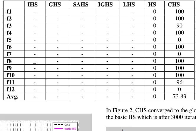
SUCCESS RATE (%)ACHIEVED BY PROBLEMShi− hij ( = 50) BY CHS AND OTHER HSVARIANT (SIGN [-]REPRESENTS NOT REPORTED IN LITERATURE)
IHS GHS SAHS IGHS LHS HS CHS
f1 - - - 0 100
f2 - - - 0 100
f3 - - - 0 90
f4 - - - 0 100
f5 - - - 0 0
f6 - - - 0 100
f7 - - - 0 0
f8 _ - - - - 0 100
f9 - - - 0 100
f10 - - - 0 100
f11 - - - 0 96
f12 - - - 0 0
Avg. - - - - - 0 73.83
Fig. 1 Convergence behaviour of CHS and basic HS algorithm on Sphere function (unimodal separable)
Conversely, basic HS took large numbers of iterations of comparable value and achieved 0% success rate.
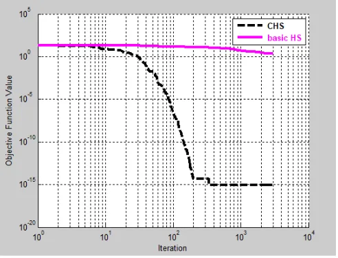
With respect to the 30-dimensional Rosenbrock function, CHS converged to the total global minimum (3.14E+01) of the function, with 0% success rate, similar to the basic HS.
In Figure 2, CHS converged to the global optimum similar to the basic HS which is after 3000 iterations.
Fig. 2 Convergence behaviour of CHS and basic HS algorithm on Rosenbrock function (unimodal non-separable)
183.86 iterations. Conversely, basic HS took large numbers of iterations of comparable value and achieved 0% success rate.
Fig. 3 Convergence behaviour of CHS and basic HS algorithm on Rastrigin function (multimodal separable)
Fig. 4 Convergence behaviour of CHS and basic HS algorithm on Ackley function (unimodal non-separable)
In the 30-dimensional Ackley function, CHS converged to the total global minimum (4.37E-15) of the function, with 100% success rate, much faster than basic HS. It is seen in Figure 4 that CHS converged to the global optimum after 164.94 iterations. Conversely, basic HS took large numbers of iterations of comparable value and achieved 0% success rate.
In conclusion, our proposed local search mechanism (CHS) is able to improve the convergence speed of basic HS and the quality of the solutions with an almost 100% success rate without getting trapped in the local optima.
IV.CONCLUSIONS
This paper presents Cosine Harmony Search (CHS) as a new modification of the Harmony Search (HS) algorithm. Our proposed algorithm introduces an additional strategy rule of parameter determination with the inclusion of a
cosine parameter multiplied by b] and b*. This increases the independence of self-modification of pitch tuning. This modification allows the algorithm to perform efficiently in both unimodal and multimodal functions.
Based on these observations, the proposed method was compared with basic HS, IHS, GHS, SAHS, IGHS and LHS. All state-of-the-art algorithms were executed with our proposed environment in 30 and 50 dimensions. The numerical results indicated that CHS offers superior performance to the existing methods on hk benchmark function. It is notable that CHS exceeds the basic HS, IHS, GHS and IGHS while the search space was increased at 50 dimensions.
It is interesting to note that although LHS performed superiorly to other HS variants in all test functions, CHS successfully achieved near global optimal solution obtained by LHS on 6 test functions, hn− ho and hm− hii at 30 dimensions, and 5 test functions, hn− ho and hm− hip at 50 dimensions. Thus, CHS performance is comparable to that of the current state-of-the-art
Furthermore, the SR average of CHS is better than basic HS, IHS, GHS and SAHS at 30 dimensions with a score of 75% in terms of reliability. When the number of dimensions is increased, CHS is still able to perform better than basic HS. Metaheuristic algorithm is successfully applied for image segmentation application [24, 25]. In line with this, it is possible that CHS which uses metaheuristic algorithm can be applied in image segmentation in the future.
NOMENCLATURE
Greek letters
, › Lower bounds of the decision variables , œ Upper bounds of the decision variables
, œ The th decision variable of the new harmony ,-.DE Minimum adjusting rate
,-.DFG Maximum adjusting rate &'DE Minimum bandwidth
&'DFG Maximum bandwidth
™.ž The value of HMCR in the th iteration New harmony vector
Var(x) The variance of the population ,-.ž The value of PAR in the th iteration
A random number uniformly distributed over the range [0,1]
Problem dimension
< 9: Worst harmony vector in the current HM
Subscripts
HM Harmony Memory
HMS Harmony Memory Size
HMCR Harmony Memory Consideration Rate PAR Pitch Adjusting Rate
BW Bandwidth
ACKNOWLEDGMENT
REFERENCES
[1] Geem, Z.W., J.H. Kim, and G.V. Loganathan. 2001. A new heuristic optimization algorithm: harmony search. simulation. 76(2): p. 60-68. [2] Liu, L. and H. Zhou. 2013. Hybridization of harmony search with
variable neighborhood search for restrictive single-machine earliness/tardiness problem. Information Sciences. 226: p. 68-92. [3] Arul, R., G. Ravi, and S. Velusami. 2013. Chaotic self-adaptive
differential harmony search algorithm based dynamic economic dispatch. International Journal of Electrical Power & Energy Systems. 50: p. 85-96.
[4] Poursalehi, N., A. Zolfaghari, and A. Minuchehr. 2013. Differential harmony search algorithm to optimize PWRs loading pattern. Nuclear Engineering and Design. 257: p. 161-174.
[5] Ahmad, I., et al. 2012. Broadcast scheduling in packet radio networks using Harmony Search algorithm. Expert Systems with Applications. 39(1): p. 1526-1535.
[6] Al-Betar, M.A., A.T. Khader, and M. Zaman. 2012. University course timetabling using a hybrid harmony search metaheuristic algorithm. IEEE Transactions on Systems, Man, and Cybernetics, Part C (Applications and Reviews). 42(5): p. 664-681.
[7] Oliva, D., et al. 2013. Multilevel thresholding segmentation based on harmony search optimization. Journal of Applied Mathematics. 2013. [8] Chun, L.B.W.F.C. and H.H.D. Xuzhu. 2013. Harmony Search Algorithm for Solving Fault Location in Distribution Networks with DG [J]. Transactions of China Electrotechnical Society. 5: p. 040. [9] Geem, Z.W., K.S. Lee, and Y. Park. 2005. Application of harmony
search to vehicle routing. American Journal of Applied Sciences. 2(12): p. 1552-1557.
[10] dos Santos Coelho, L. and V.C. Mariani. 2009. An improved harmony search algorithm for power economic load dispatch. Energy Conversion and Management. 50(10): p. 2522-2526.
[11] Ouyang, H.-b., et al. 2017. Improved Harmony Search Algorithm: LHS. Applied Soft Computing. 53: p. 133-167.
[12] Worasucheep, C. 2011. A harmony search with adaptive pitch adjustment for continuous optimization. International Journal of Hybrid Information Technology. 4(4).
[13] Mahdavi, M., M. Fesanghary, and E. Damangir. 2007. An improved harmony search algorithm for solving optimization problems. Applied mathematics and computation. 188(2): p. 1567-1579.
[14] El-Abd, M. 2013. An improved global-best harmony search algorithm. Applied mathematics and computation. 222: p. 94-106. [15] Omran, M.G. and M. Mahdavi. 2008. Global-best harmony search.
Applied mathematics and computation. 198(2): p. 643-656. [16] Wang, C.-M. and Y.-F. Huang. 2010. Self-adaptive harmony search
algorithm for optimization. Expert Systems with Applications. 37(4): p. 2826-2837.
[17] Jaddi, N.S. and S. Abdullah. 2017. A cooperative-competitive master-slave global-best harmony search for ANN optimization and water-quality prediction. Applied Soft Computing. 51: p. 209-224. [18] Ayob, M., et al. 2013. Enhanced harmony search algorithm for nurse
rostering problems. Journal of Applied Sciences. 13(6): p. 846-853. [19] Yassen, E.T., et al. 2015. Meta-harmony search algorithm for the
vehicle routing problem with time windows. Information Sciences. 325: p. 140-158.
[20] Turky, A., S. Abdullah, and A. Dawod. 2018. A dual-population multi operators harmony search algorithm for dynamic optimization problems. Computers & Industrial Engineering. 117: p. 19-28. [21] Jurjee, M.M.J., et al. 2017. Multi-Population Harmony Search
Algorithm For The Dynamic Travelling Salesman Problem With Traffic Factors. Journal of Theoretical & Applied Information Technology. 95(2).
[22] Shatnawi, M., M.F. Nasrudin, and S. Sahran. 2017. A new initialization technique in polar coordinates for Particle Swarm Optimization and Polar PSO. International Journal on Advanced Science, Engineering and Information Technology. 7(1): p. 242-249. [23] Hussein, W.A., S. Sahran, and S.N.H.S. Abdullah. 2014. Patch-Levy-based initialization algorithm for Bees Algorithm. Applied Soft Computing. 23: p. 104-121.
[24] Hussein, W.A., S. Sahran, and S.N.H.S. Abdullah. 2016. A fast scheme for multilevel thresholding based on a modified bees algorithm. Knowledge-Based Systems. 101: p. 114-134.