An Assessment of the Option to Reduce the Investment in a Project by the Binomial
Pricing Model
Salvador Cruz Rambaud, Ana Maria Sanchez Perez
University of Almeria
Ctra. Sacramento, s/n, 04120 La Canada, Almeria, Spain E-mail. [email protected], [email protected]
http://dx.doi.org/10.5755/j01.ee.28.5.17636
Real options are a powerful complement to traditional methods of investment project assessment, such as the Net Present Value, when the value of some business strategies has to be included. This paper presents a methodology to calculate the value of the real option to reduce the productive capacity of an investment project within one, two, and n periods. It is well known that the option to reduce quantifies the value of the operational flexibility available to protect a business against possible losses generated by the project; its common use in business practice explains the relevance of developing a clear and easy-to-use tool to assess its value. Thus, to derive its value, the procedure implemented here consists of obtaining a mathematical expression for each of the aforementioned periods, based on a detailed construction of every possible future scenario and its associated probability by the multiplicative binomial method. This is a useful contribution to business practice as it provides a well-defined model to assess the strategic value of an investment project including the option to reduce its productive capacity. Moreover, this real option increases the project value by improving its initial level of feasibility.
Keywords: Real Option, Option to Reduce, Binomial Pricing Model, Investment Project Assessment, Financial Engineering.
Introduction
The improvement of asset valuation models is one of the prevailing trends in current research in financial theory. In effect, traditional methods for assessing investment projects are substantially limited when implicit uncertainty factors are involved. Moreover, they are based on the estimation of a single scenario, where only one strategy is considered, leaving aside the possible implications of different strategies in the maximization of the Net Present Value (NPV) of the project in the medium and long term (Santos et al., 2014).
During the period covered by a given cash flow, some of the initial uncertainties may disappear (Park and Herath, 2000). When this happens, the decision-maker becomes an active agent who can alter the project strategy to adapt to changing market conditions. In this way, the investment should be considered as a continuous process of identification, selection and implementation of opportunities (Bernardo and Chowdhry, 2002).
The employment of the discounted cash flow model may underestimate the benefits of the project, because the project value is not only defined by its associated cash flows (Merlo, 2016). The value of flexibility is of significant importance for projects with high volatility (where it is likely that further relevant information may be received in the future) and whose expected NPV is near 0. Under these circumstances, the flexibility provided by real options must necessarily be taken into account (Nicholls et al., 2014).
Since the majority of companies operate in uncertain environments, the possibility of modifying the initial strategy means a new source of added value. Therefore, different strategies must be regularly considered, and this flexibility should be reflected in the project value. In this context,
Myers (1984) introduces the dynamic NPV which includes the traditional NPV plus the real option value.
Traditionally, a high level of uncertainty has had a negative impact when evaluating a project, but this situation can also be viewed as a source of new opportunities. In this way, Shil and Allada (2007) argue that uncertainties should be integrated in the evaluation model. Thus, the use of real options shows that a correct management of uncertainty may add value to the project if managers are able to identify and use the option to respond to new circumstances as they arise. The analysis and assessment of real options allow for the incorporation of strategic aspects such as operational flexibility, the adaptability to the market or the strategic value of the project. The option value plus the project NPV give rise to a total NPV, where the project may be justified if the total NPV is greater than zero (Nicholls et al., 2014). Therefore, those new circumstances may change the viability of an initially non-viable project, valued by a traditional appraisal method, even making it highly profitable (Koller, 2005; Metelski et al., 2014). In summary, the main contribution of the real option theory is the incorporation of strategic aspects in the assessment of a project and the introduction of the idea that uncertainty may be related to the creation of opportunities.
In Block (2007) it is revealed that the percentage of companies which use real options is small but growing in recent years. Real options have been studied by numerous authors from an applied point of view, especially in the energy sector (Kim et al., 2016; Torani et al., 2016; Fernandes et al., 2011; Schachter & Mancarella, 2016; Secomandi & Seppi, 2014; Bastian-Pinto et al., 2010) and the information and communications technology (ICT) sector (Chen et al., 2009; Cassimon et al., 2011; Harmantzis and Tanguturi, 2007). In this way, “some top managers and consultants would like to use real options as a rhetorical tool that can be used to justify investment, financing and acquisition decisions; they feel that while there are embedded options in most decisions, they cannot be valued with any precision. There are others who argue that we should try to quantitatively estimate the value of these options, and build them into the decision process” (Damodaran, 2012).
In this way, the aim of this paper is to introduce a novel method for assessing an investment project including the option to reduce its scale of production. The option to shut down a part of the project always has a value higher than or equal to 0 because it provides the flexibility to soften possible future losses. In this case, this option increases the value of the project because the investor is protected from further losses when the result of uncertainty is unfavorable for the project (McDonald and Siegel, 1985). Consequently, if a company decides to operate with a smaller productive capacity, part of the investment can be recovered with the purchase of a part of the project’s residual value. In this paper, the importance of the residual value is stressed, since previous research estimates the future cash flows using a value without any given justification.
The option to reduce investment in a project is particularly valuable when new products are launched in uncertain markets (Hagspiel et al., 2016), or when using new technologies (Kauffman & Li, 2005) or plant designs with different cost structures and maintenance costs.
The methodology employed in this paper is based on the binomial pricing model (Copeland & Antikarov, 2003), one of the most well-known models for evaluating financial options. Given the conceptual similarities between financial (put) options and real (option to reduce) options, Amram and Kulatilaka (1999) implement the methodology for real-option valuation as an extension of that of financial real-options (Seifert, 2015).
In summary, this paper aims to answer the following research question: in unstable environments, do the companies have any tools to assess the strategic value of reducing their productive capacity? To do this, we derive the expression of the option to reduce an investment project by using the multiplicative binomial model. Moreover, we prove that, as expected, the option value is always greater than or equal to zero and that, as the option maturity increases, the value of the option to reduce also increases. In Section 2 the expression of the options to reduce within one, two and n periods are respectively deduced. In Section 3 the significance of our findings are discussed. Finally, Section 4 summarizes and concludes.
Valuing the Option to Reduce a Project
In general, the net present value of a project with the option to reduce within n periods (denoted by ()
0
)
(
nR
V
) is, by using continuous stochastic processes:, d
d ) , (
} , ) 1 ( { max )
1 (
1 )
(
0 ) ( ) (
) ( )
( 0
I A V A V f
V A V
r R
V
n R n n R n
n n R n
n f n
(1)
where:
n is the duration of the project.
r
f is the risk-free interest rate. Vn is the random variable which describes the project value (without taking into account the initial investment) at moment n. That is:
, , , 2 , 1 , ) 1 ( 1
N n
k x V
N
i
i n i
n
(2) where xi is the cash flow of the project at instant i
) , , 2 , 1
(i N and N the finite life-span of the project. A priori, N is considered to be finite; but this question is not relevant in the calculations because all cash flows are included in the expression of Vn.
is the percentage by which the cash flows would be diminished after the reduction. (n)
R
A is the residual value of a part of the investment project at instant n.
( , (n))
R n A V
f is the joint probability density function of Vn and
) (n R A .
I0 is the initial investment which is necessary to
set the project in motion.
In order to determine expression (1), we will specify each one of its parameters. First, we will use as stochastic financial process the binomial options pricing model. We will then derive the residual value of the project at instant n (denoted by RVn) as a first step to calculating the purchase price of a part of the project at that instant. In this way, according to the Gordon and Shapiro (1956) model, the residual value of the project can be calculated as follows:
, ) 1 (
g k
g x
RV n
n
(3)
where k is the market discount rate and g the cumulative increase rate of cash flows. In Copeland et al. (2010) the value of the lager company Heineken is studied in detail. More specifically, its residual value is calculated as an infinity annuity by employing equation (3).
If the cash flows produced by the project are the components of the random vector (x1,x2,...,xN), Vn is a random variable whose variance is given by the following expression:
. ) , cov( )
1 ( 2 ) ( ) 1 ( ) (
1
2 1
2 ) ( 2
2
N j i
j i j i n N
i
i i n
n k x k x x
V
likely to be less permanent that positive cash flows […]. Consequently, holding constant the expected level of cash flows from existing projects or divisions, cash flow volatility should be positively related to future cash flows”. Thus, taking into account that the random cash flows
N x x
x1, 2,..., are produced within the life-span of the project, it is expected that all covariances are positive, for every i and j such that 1i jN. Thus, the relationship between the volatilities of Vn and xi is obviously:
. 1 , 1
), ( )
(Vn xi nN in
Therefore, if t is the length of the time interval in which the project value changes, one has (Hull, 1989):
i i
n t x t u
V
uexp{
( ) }exp{
( ) }: and, consequently, if xi is going to follow a dichotomous random variable, then
. i u u
On the other hand, the parameter di can be determined starting from the value of ui, the volatility of the i-th cash flow and the probabilities p and q. Observe that, in general,
i i
u d
1 . In general terms, it is logical to assume that the
range of possible values of the residual value should be less than the corresponding range of the project value (Kogut and Kulatilaka, 2004). This statement is in line with Mascareñas (2004): if things go well, an early abandonment of the project is not the best decision, but if they go badly, it might be advisable. Finally,
, ) 1 )( 1 ( ) ( ) 1 )( ( )
( 0 1
g k
g r x
E
g k
g x E RV
E i
n
i n
n
where 1ri: puiqdi is the average increasing factor of the i-th cash flow. However, in this paper we are going to assume that the volatility of cash flows is constant during the project’s life-span, whereby we can take
1 ) 1 (
/ 1
1
N N
i i r
r as the average increase of the
residual value. Therefore, we can write:
, ) 1 ( ) 1 ( ) 1 )( ( )
( 0 0 n
n
n RV r
g k
g r
x E RV
E
where
g k
g x E RV
( 0)(1 )
0 is the residual value at moment
0, where g can be taken asrf. Taking into account that the project is assumed to be feasible, the expected increase in cash flow must be greater than the risk-free interest rate, so the following inequality holds:
,
f
r
r
where 1r:puqd. Therefore, if RVn is going to follow a dichotomous random variable with the same probabilities of occurrence p and q, and where obviously
N
i i u u
1
then
. u u
The two former inequalities easily show that d
d
and so
RV
n
,
1
RV
nu
with probabilityp,
1
RV
nd
with probabilityqwhere uudd.
Option to reduce within one period
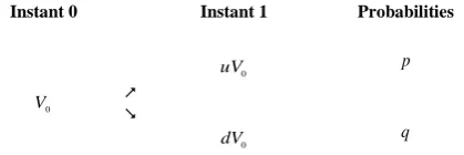
In this subsection, we are going to calculate the value of the option to reduce within one period. As indicated, the methodology for the analysis of the evolution of the project value and its residual value is the binomial distribution. Figure 1 shows the evolution of the project value for one period.
Moreover, Figure 2 shows the evolution of the residual value of a part of the project for one period.
Figure 2. Evolution of the residual value of a part of the project
within one period. Source: Own elaboration.
In this way, expression (1) will accept only the following possible values:
In the case of a favorable evolution of the project:
}. 0 , max{
} , ) 1 ( max{
0 ) 0 ( 0
0 ) 0 ( 0
V u A u uV
uV A u uV
V
R R
Otherwise, if the evolution is unfavorable:
}. 0 , max{
} , ) 1 ( max{
0 ) 0 ( 0
0 ) 0 ( 0
V d A d dV
dV A d dV
V
R R
Therefore, the project value with the option to reduce will depend on the relative position of the residual value of a part of the investment with respect to the possible evolution of the corresponding project value. Observe that this relationship may also be established between the project value and its residual value. More specifically:
} 0 ,
max{ 0 0
0 uRV uV
uV
V
and
}. 0 ,
max{ 0 0
0 dRV dV
dV
V
Consequently, the project value with the option to reduce in one period is:
. 1
)
( (1) 0
0 I
r qV pV R V
f
Instant 0 Instant 1 Probabilities
0
uV p
0
V
0
dV q
Figure 1. Evolution of the project value within one period.
Source: Own elaboration.
Instant 0 Instant 1 Probabilities
) 0 (
R
A
u p
) 0 (
R
A
) 0 (
R
A
As
u
RV
0
uV
0, it can be deduced thatV
uV
0
, whilst
V can take two values, depending on the relative position of
d
RV
0 anddV
0. Summarizing:
V
uV
0
V
Therefore, the expression of the project value with the option to reduce within one period remains as follows:
) 1 ( 0)
(
R
V
,
0
0 I
V if 0 V0
d d RV
, 1
) (
0 0 0
0 I
r dV RV d q V
f
if 0 V0
d d RV
After analyzing the project value with the option to reduce within a single period, we will prove mathematically that, as expected, its value is greater than or equal to the value of the project without this option. The final objective will be obtaining the value of the option to reduce.
Proposition 1. The present value of an investment project with the option to reduce within a single period is always greater than or equal to V0I0.
Proof. We will analyze the following two cases:
1. If 0 V0
d d RV
, the present value of the investment project with the option to reduce is:
, 1
)
( (1) 0 0 0 0 0
0 I V I
r qdV puV R
V
f
which confirms the statement of the proposition. 2. If 0 V0
d d RV
, the present value of the project with the option to reduce is:
) 1 ( 0)
(
R
V
,1
) (
0 0 0
0 I
r dV RV d q V
f
which is obviously greater than V0I0. □
Some comments arising from this result:
If 0 V0
d d RV
, the decision to reduce is irrelevant because the selling price of the part of the project to reduce does not exceed the value of the cash flows generated by this part of the project under the most adverse conditions. Thus, the project’s present value, V0I0, is not affected by the
reduction, since as a consequence the option value is equal to zero.
On the other hand, if 0 V0
d d RV
, the amount obtained from the sale of part of the project is in an intermediate position between the project value
in the most favorable situation and that obtained in the less favorable. In this case, the option value is positive.
Once the expression of the option to reduce has been derived, we will apply the developed model to a numerical example based on an investment project promoted by an oil company. The information is given in millions of euros:
Initial investment, I0104.
Present value of the project, V0100. Risk-free discount rate, rf 5%.
Up and down factors affecting the project value, 8
. 1
u and d = 0.56, respectively. It is well known that the risk-neutral probabilities can be calculated by using the following expressions:
d u
d r
p f
(1 ) and q1p,
from where p39.5% and
% 5 . 60 1
p
q .
Up and down factors affecting the residual value, 5
. 1
u and d0.9, respectively. As indicated, these factor values do not satisfy the rule
u d
1
given that its values are considered as given by estimations. To work with these values, it has been considered that the project volatility is constant throughout the duration of the project.
The project has the option to reduce its production capacity at the end of the first period by 30% (
0.30).Thus, the value of the project with the option to reduce within a single period is given by the following piece-wise function:
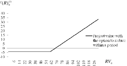
whose graphic representation according to the residual value is (see Figure 3):
Figure 3. Project value with the option to reduce within one
period. Source: Own elaboration.
,
0
dV if
0
0
dV
RV
d
),
(
0 00
d
RV
dV
dV
ifdV
0
d
RV
0, 4
if
RV
0
62
.
22
, 4 05
. 1
) 56 9
. 0 ( 1815 .
0 RV0
if
RV
0
62
.
22
) 1 ( 0
) (R V
0
RV
) 1 ( 0
Once the value of the project with the option to reduce in one period has been obtained, the value of the option can be deduced using the following formula:
0 0 )1 ( 0
)
(
R
V
I
V
(1)R O .
Corollary 1. The mathematical expression of the value of the option to reduce within one period (denoted by (1)
R O ) is:
Proof. The proof is obvious for each case, as it is only necessary to find the difference between the project value with the option,
V
(
R
)
(01), and the project value without it,0
0 I
V (see the proof of proposition 1):
:
(
)
(
0 0)
) 1 ( 0 )
1 (
I
V
R
V
O
R
. □In Example 1, the value of the option to reduce within one period results in:
) 1 (
R O
0, if
62
.
22
0
RV
,
68
.
9
1556
.
0
RV
0
ifRV
0
62
.
22
The graphical representation is depicted in Figure 4.Figure 4. Value of the option to reduce within one period.
Source: Own elaboration.
Option to Reduce Within Two Periods
In order to calculate the present value of an investment project with the option to reduce within two periods (denoted by (2)
0
)
(
R
V
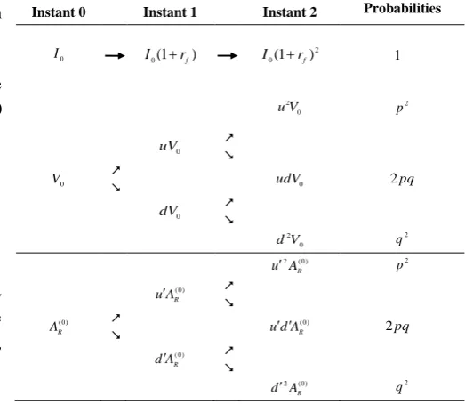
), we should take into account (see Figure 5): the evolution of the residual value previous to the sale of a part of the project at the end of the second period, and
the evolution of the value corresponding to the percentage of the project to be reduced.
Figure 5. Evolution of the initial payment, project value and residual value within two periods.
Source: Own elaboration.
Therefore, the possible values of the project within two periods are given by the following expressions:
}, 0 , max{
} , )
1 ( max{
0 2 ) 0 ( 2 0
2
0 2 ) 0 ( 2 0
2
V u A u V
u
V u A u V
u V
R R
} 0 , max{
} , )
1 ( max{
0 )
0 ( 0
0 ) 0 ( 0
V ud A d u udV
udV A d u udV
V
R R
and
}, 0 , max{
} , )
1 ( max{
0 2 ) 0 ( 2 0
2
0 2 ) 0 ( 2 0
2
V d A d V
d
V d A d V
d V
R R
with their probabilities of occurrence being 2
p , 2pq and
2
q , respectively. Therefore, the present value of the project with the option to reduce is the discounted mathematical expectation:
,
) 1 ( 2 )
( 2 0
2 2
) 2 (
0 I
r
V q pqV V
p R V
f
(4) where V, V and V are functions of
RV
0 andV
0 , such that:},
0
,
max{
02 0 2 0
2
V
u
RV
u
V
u
V
}
0
,
max{
0 00
u
d
RV
udV
udV
V
and
}
0
,
max{
02 0 2 0
2
V
d
RV
d
V
d
V
.In this way and based on Equation (4), we can obtain the project value depending on the residual present value position with respect to certain limits. Since uu and
0
0 V
RV , it is verified that 0 2 0 2
V
u
RV
u
. So, we can write:,
0 2
V
u
V
[1]0, if 0 V0
d d RV
, 1
)
( 0 0
f r
dV RV d q
if 0 V0
d d RV
Instant 0 Instant 1 Instant 2 Probabilities
0
I I0(1rf)
2 0(1 rf)
I 1
0 2
V
u 2
p
0
uV
0
V
udV0 2pq
0
dV
0 2
V
d 2
q
) 0 ( 2
R
A
u 2
p
) 0 (
R
A
u
)
0 (
R
A
) 0 (
R
A d
u 2pq
) 0 (
R
A
d
) 0 ( 2
R
A
d 2
q
) 1 (
R O
0
RV
) 1 (
R
Therefore, we must bear in mind the following cases: 1. If inequality [4] holds, since dd, it implies that
0
0 dV
RV
d ; and since uu the inequality [2] also holds. That is to say, [4] necessarily implies [2]:
02 0 2
V
d
RV
d
u
d
RV
0 udV
0. 2. Ifd
2V
0
d
2RV
0 (inequality [5]),u
d
RV
0
udV
0may occur, that is, inequality [2].
3. Finally, if
udV
0
u
d
RV
0 , then 0 2 0 2RV
d
V
d
.That is to say, [3] necessarily implies [5]:
00
u
d
RV
udV
02 0 2
RV
d
V
d
.Thus, the project value with the option to reduce within two periods, according to these three cases and their corresponding implications, is the following:
* ,
) 1 (
) (
0 2
0 2 0 2 2
0 I
r V d RV d q V
f
** ,
) 1 (
) (
) (
2
0 2
0 2 0 2 2 0 0
0 I
r
V d RV d q udV RV d u pq V
f
In the rest of this Section and with the final objective of obtaining the value of the option to reduce the project within two periods, we are going to demonstrate mathematically that the present value of the investment project with the option to reduce within two periods is greater than or equal to the project value without this option and, moreover, greater than or equal to the project value with the option to reduce within one period.
Proposition 2.
(
)
(
)
0 0.
) 1 ( 0 )
2 (
0
V
R
V
I
R
V
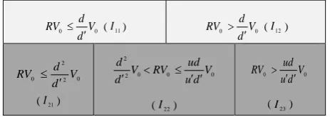
Proof. For a better understanding of this demonstration, Figure 6 specifies the possible intervals to which
RV
0 can belong when the option to reduce is in asingle period (I1n, where n = 1 and 2; in light grey) and when it is in two periods (I2n, where n = 1, 2 and 3; in dark grey).
0
0 V
d d RV
(I11) 0 V0
d d RV
(I12)
0 2 2
0 V
d d RV
(I21)
0 0 0 2 2
V d u
ud RV V d d
(I22)
0
0 V
d u
ud RV
(I23)
Figure 6. Possible intervals for RV0 when the option to reduce
is within one or two periods.Source: Own elaboration.
First, we are going to demonstrate that, in Figure 6, the position of
RV
0 in any interval of period 2 implies its belonging to the intervals of period 1 specified in the cells immediately above. In effect,1. If 2 0,
2
0 V
d d RV
then 2 0 0,
2
0 V
d d V d
d RV
because 1
d d
. Therefore, I21 implies I11.
2. If 2 0 0 0,
2
V d u
ud RV V d
d
a priori there could be
any relationship of inequality between
RV
0 and0
V d d
. Therefore, I22 implies I11I12.
3. If V0 RV0,
d u
ud
then 0 V0 RV0,
d u
ud V d
d
since 1
u u
. So, I23 implies I12.
The proof of the proposition is demonstrated as follows:
1. If 2 0,
2
0 V
d d RV
the project value is not affected by the option to reduce. Therefore,
, )
( 0 0
) 2 (
0 V I
R
V
satisfying, in this way, the required equality/inequality.
2. If 2 0 0 0
2
V d u
ud RV V d
d
, the present value of the
investment project with the option to reduce within two periods is:
) 2 ( 0)
(
R
V
.) 1 (
) (
0 2
0 2 0 2 2
0 I
r V d RV d q V
f
Since 0
2 0 2
RV
d
V
d
, it can be proved that )2 ( 0
)
(
R
V
is greater than or equal to the project value without the option to reduce within two periods; and greater than or equal to the project value with the option to reduce in a single period when0
0 V
d d RV
. That is to say:
V
,
0
udV if
u
d
RV
0
udV
0 [2]),
( 0 0
0 udRV udV
udV if
udV
0
u
d
RV
0 [3]
V
,
0 2
V
d
if 02 0 2
V
d
RV
d
[4]),
(
02 0 2 0 2
V
d
RV
d
V
d
ifd
2V
0
d
2RV
0 [5],
0
0 I
V if 2 0
2
0 V
d d RV
* if 2 0 0 0
2
V d u
ud RV V d
d
** if 0 V0
d u
ud RV
.
)
(
)
(
0 0) 1 ( 0 ) 2 (
0
V
R
V
I
R
V
It remains to prove the former inequality when
0 0 V d d RV
. In this case,
) 1 ( 0)
(
R
V
. 1 ) ( 0 0 0 0 I r dV RV d q V f As
r
r
f, thenf f r u p r d q 1 1
1 and so the
following chain of inequalities holds:
) 2 ( 0)
(
R
V
2 0
0 2 0 2 2 0 ) 1 ( ) ( I r V d RV d q V f
0 0 0
0 1 1 1 1 1
1 V I
r qd r pu RV r d q r u p V f f f f . ) 1 ( 1 ) 1 ( 1 0 0 2 0 0 2 0 0 I V r pqud V r qd RV r d u pq RV r d q V f f f f
As
u
d
RV
0
udV
0, then
) 2 ( 0)
(
R
V
(1)0
)
(
R
V
.3. If 0 V0
d u ud RV
, the present value of the project with the option to reduce within two periods is:
0 0
) 2 ( 0 )
(R V I
V . ) 1 ( ) ( ) ( 2 2 0 2 0 2 2 0 0 f r V d RV d q udV RV d u pq
As
udV
0
u
d
RV
0 then 2 0 02
RV
d
V
d
and so0 0 ) 2 ( 0 )
(R V I
V . On the other hand, as
0 0 V d d RV
, then:
) 1 ( 0)
(
R
V
. 1 ) ( 0 0 0 0 I r dV RV d q V f In this case,
V
(
R
)
(02) can be rewritten as follows:, ) 1 ( ] ) [( ] ) [( ) ( 2 0 2 2 2 0 2 2 0 0 ) 2 ( 0 f r V u p qd pu RV u p d q u p I V R V
2 0 0 0 0 ) 2 ( 0 ) 1 ( ] ) 1 [( ] ) 1 [( ) ( f f r V qd pu r RV d q u p r I V R V
, . ) 1 ( ] ) 1 [( ] ) 1 [( ) ( 2 0 0 0 0 ) 2 ( 0 f f r RV pqud qd r RV d u pq d q r I V R V
As
r
r
f and udRV0udV0, then:
0 2 0 0
0 ) 2 ( 0 ) 1 ( ) 1 ( ) 1 ( ) ( I r V qd r RV d q r V R V f f
f
. ) ( 1
)
( (1)
0 0
0 0
0 I V R
r dV VR d q V f
□In Example 1, the project value with the option to reduce within two periods is determined by the following piece-wise function:
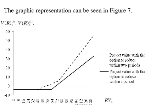
The graphic representation can be seen in Figure 7.
Figure 7. Project value with the option to reduce within one and
two periods. Source: Own elaboration.
Figure 7 confirms Proposition 2, since the project value with the option to reduce within two periods is always greater than or equal to the project value with the option to reduce in a single period.
Corollary 2. The value of the option to reduce within two periods (denoted by (2)
R O ) is:
2 0 2 0 2 2 0 0 ) 1 ( ) ( ) ( 2 * f r V d RV d q udV RV d u pq
Proof. The proof is obvious for each case (for more
details see the proof of Proposition 2). □ With the data of Example 1, the value of the option to
reduce within two periods is:
4, if RV0 38.727.123, 0807
.
0 RV0 if 38.72RV0 74.67 ,
233 20 256
0. RV0 . if RV0 74.67
,
0 if 2 0
2 0 V d d RV , ) 1 ( ) ( 2 0 2 0 2 2 f r V d RV d q
if 2 0 0 0
2 V d u ud RV V d d
* if V0 RV0
d u ud ) 2 ( 0 ) (R V 0 RV , ) ( , )
( (2)
0 ) 1 (
0 V R
The graphic representation is (see Figure 8):
Figure 8. Value of the option to reduce in one and two periods.
Source: Own elaboration.
Option to Reduce Within n Periods
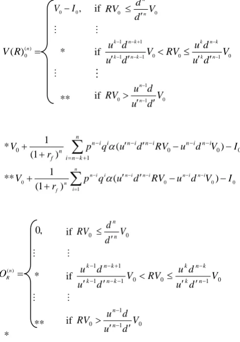
The present value of the investment project with the option to reduce within n periods
(
(
)
())
0
n
R
V
, and the value of the related option to reduce (denoted by (n)R
O ) are the following:
* 0 0
1
0
0 ( )
) 1 (
1
I V d u RV d u q p r
V n i n i
n
k n i
i n i n i i n n f
** 0 0
1
0
0 ( )
) 1 (
1
I V d u RV d u q p r
V ni ni
n
i
i n i n i i n n f
*
) (
) 1 (
1
0 1
0 u d V
RV d u q p r
i n i n n
k n i
i n i n i i n n f
** ( )
) 1 (
1
0 1
0 u d V
RV d u q p r
i n i n n
i
i n i n i i n n f
Discussion
This work aims to provide managers and professionals from different sectors with some easy-to-use tools to assess real options. In effect, the high level of sophistication and low functionality of most models may explain why they are rarely used in business practice.
The main contribution of this paper is the introduction of a theoretical and detailed development of the binomial options pricing model applied to assess the value of the real option to reduce the productive capacity of an investment project.
This new model derivation has been explained in detail by considering different time horizons. It has been proved that the value real option to reduce is directly related to its duration (it is also graphically shown in Figure 7). In this way, the value of the real option to reduce exhibits a similar behavior to the value of the call and put financial options (Black and Scholes, 1973). This relationship makes sense given that the value of the option increases with the increase of the duration of the project.
Our approach does not aim to replace the widely used Net Present Value but, on the contrary, it is an extension. The practical importance of the model in business is remarkable as it allows making a distinction between a financial analysis (the project value based on its future cash flows) and the strategic one (the project value which includes some future strategic opportunities). As a consequence, the implementation of this model makes it easier for companies to consider real options, and thereby to increase their competitiveness.
Nevertheless, the practical application of this methodology has several limitations such as:
As in traditional assessment methods, the necessary information to apply the model may not be available or might be predicted in an inappropriate way. This has a negative impact on the result of the assessment. To solve it, companies should address their efforts to the realization of their own forecasts.
Its effective application requires considering a detailed analysis of all possible cases.
Traditionally, the option to reduce a project investment has been calculated, for example, in the energy or mining sectors in which this kind of real option is very common and may play a fundamental role. Nevertheless, the use here of the well-known Black-Scholes model does not provide an incremental accuracy which can justify the use of this sophisticated model.
Conclusions
In view of the under-implementation of the methodologies to quantify real options in business practice, despite the undeniable importance of their inclusion in the
0 , if RV0 38.72
3.123, 0807
.
0 RV0 if 38.72RV0 74.67
, . RV
.256 13233
0 0 if RV0 74.67
,
0
0 I
V if 0 V0
d d RV
n n
* if 1 1 0 0 1 0
1 1
V d u
d u RV V d u
d u
n k
k n k
k n k
k n k
** if 1 0
1
0 V
d u
d u
RV n
n
,
0 if 0 V0
d d
RV n
n
* if 0
1 0
0 1 1
1 1
V d u
d u RV V d u
d u
n k
k n k k
n k
k n k
** if 1 0
1
0 V
d u
d u
RV n
n
) 2 (
R O
0 RV )
2 ( ) 1 (
, R
R O
O
) ( 0 )
( n
R V
assessment of investment projects, this paper aims to provide a simple formula to quantify the value of the option to reduce.
The methodologies employed to assess real options based on continuous models are complex, and consequently most managers and business people are reluctant to use them. The binomial pricing model, however, is simpler and hence more manageable.
In order to improve the managerial decision, it is necessary to increase the use of option pricing models. The contribution of this paper is the presentation of a single expression for quantifying the value of the option to reduce, supplementary to the NPV formula, in order to obtain the total value of the project.
Our formulation is based on the mathematical implementation of the binomial pricing model. The
procedure consists in the construction of two main estimates: the basic project value and the project value with the flexibility to change the company strategy, that is to say, with the real option included. The expression to obtain the value of the option of reducing the project in one, two or n periods offers the possibility to realize a more accurate assessment of the project through the integration of intangible aspects in its value. Finally, this paper proves that the value of a project with the option to reduce increases with respect to time.
As a line of future research, we highlight the possibility to elaborate a guide capable of making easier the implementation of this model and of identifying all possible cases which may arise in the assessment of the option to reduce a project investment.
References
Amram, M., & Kulatilaka, N. (1999). Real Options: Managing Strategic Investment in an Uncertain World. Boston: Harvard Business School Press.
Bastian-Pinto, C., Brandao, L., & De Lemos Alves, M. (2010). Valuing the Switching Flexibility of the Ethanol-Gas Flex Fuel Car. Annals of Operations Research, 176 (1), 333–348. doi: 10.1007/s10479-009-0514-7.
Bernardo, A. E., & Chowdhry, B. (2002). Resources, Real Options and Corporate Strategy. Journal of Financial Economics, 63, 211–234. doi.org/10.1016/S0304-405X(01)00094-0.
Black, F., & Scholes, M. (1973). The Pricing of Options and Corporate Liabilities. Journal of Political Economy, 81(3), 637–654. doi.org/10.1086/260062.
Block, S. (2007). Are “Real Options” Actually Used in the Real World?. The Engineering Economist, 52(3), 255–267. doi.org/10.1080/00137910701503910.
Cassimon, D., Engelen, P. J., & Yordanov, V. (2011). Compound Real Option Valuation with Phase-Specific Volatility: A Multi-Phase Mobile Payments Case Study. Technovation, 31(5), 240–255. doi.org/10.1016/j.technovation.20 10.12.004.
Chen, T., Zhang, J., & Lai, K. K. (2009). An Integrated Real Options Evaluating Model for Information Technology Projects under Multiple Risks. International Journal of Project Management, 27(8), 776–786. doi.org/10.1016/j.ijproman.2009.01.001.
Copeland, T., & Antikarov, V. (2003). Real Options: A Practitioner’s Guide. New York: Texere.
Copeland, T., Koller, T., & Murrin, J. (2010). Valuation: Measuring and Managing the Value of Companies (3rd Ed.). New
York: John Wiley and Sons, Inc.
Damodaran, A. (2012). Investment Valuation: Tools and Techniques for Determining the Value of any Asset (3rd Ed.). New
York: Wiley Finance Publishers.
De Oliveira Pamplona, E., Carvalho Brandão, M., Barra Montevechi, J. A., Ferreira De Pinho, A., Oscar Albuquerque, V., & Rotela Junior, P. (2013). Evaluating Energy Sector Investments: Calculating Volatility. Mathematical Problems in Engineering, vol. 2013, Article ID 128309, 9 pages, doi.org/10.1155/2013/128309.
Fernandes, B., Cunha, J., & Ferreira, P. (2011). The Use of Real Options Approach in Energy Sector Investments. Renewable and Sustainable Energy Reviews, 15(9), 4491–4497. doi.org/10.1016/j.rser.2011.07.102.
Gordon, M. J., & Shapiro, E. (1956). Capital Equipment Analysis: The Required Rate of Profit. Management Science, 3(1), 102–110. doi.org/10.1287/mnsc.3.1.102.
Hagspiel, V., Huisman, K. J., & Kort, P. M. (2016). Volume Flexibility and Capacity Investment under Demand Uncertainty. International Journal of Production Economics, 178, 95–108. doi.org/10.1016/j.ijpe.2016.05.007. Harmantzis, F. C., & Tanguturi, V. P. (2007). Investment Decisions in the Wireless Industry Applying Real Options.
Telecommunications Policy, 31(2), 107–123. doi.org/10.1016/j.telpol.2006.02.005.
Hull, J. C. (1989). Options, Futures and Other Derivatives (3rd Ed.). New Jersey: Prentice Hall.
Kauffman, R. J., & Li, X. (2005). Technology Competition and Optimal Investment Timing: A Real Options Perspective. IEEE Transactions on Engineering Management, 52(1), 15–29. doi: 10.1109/TEM.2004.839962.
Kogut, B., & Kulatilaka, N. (2004). Real Options Pricing and Organizations: The Contingent Risks of Extended Theoretical Domains. Academy of Management Review, 29(1), 102–110. doi: 10.5465/AMR.2004.11851725. Koller, T., Goedhart, M., & Wessels D. (2005). Valuation: Measuring and Managing the Value of Companies (4th Ed.).
Nueva York: Mckinsey.
Mascarenas, J., Lamothe, P., Lopez Lubian, F. J., & De Luna, W. (2004). Opciones Reales y Valoracion de Activos. Madrid: Prentice-Hall.
McDonald, R. L., & Siegel, D. R. (1985). Investment and the Valuation of Firms when there is an Option to Shut Down. International Economic Review, 26(2), 331–349. doi: 10.2307/2526587.
Merlo, P. (2016). Consequences of the Absence of Monotonicity of the NPV Function to the Assessment of Effectiveness of Investment Projects. Inzinerine Ekonomika-Engineering Economics, 27(1), 39–46. http://dx.doi.org/10.57 55/j01.ee.27.1.6334.
Metelski, D., Mihi-Ramirez, A., & Arteaga-Ortiz, J. (2014). Research and Development Projects upon Real Options View. Engineering Economics, 25(3), 283–293. http://dx.doi.org/10.5755/j01.ee.25.3.2737.
Myers, S. C. (1984). Finance Theory and Financial Strategy. Interfaces, 14, 126–137. doi.org/10.1287/inte.14.1.126.
Nicholls, G. M., Lewis, N. A., Zhang, L., & Jiang, Z. (2014). Breakeven Volatility for Real Option Valuation. Engineering Management Journal, 26(2), 49–61. doi.org/10.1080/10429247.2014.11432010.
Nissim D. (2002). Discussion of “The Role of Volatility in Forecasting”. Review of Accounting Studies, 7, 217–227. Park, C. S., & Herath, H. S. (2000). Exploiting Uncertainty-Investment Opportunities as Real Options: A New Way of
Thinking in Engineering Economics. The Engineering Economist, 45(1), 1–36. doi.org/10.1080/00137910008967534. Santos, L., Soares, I., Mendes, C., & Ferreira, P. (2014). Real Options versus Traditional Methods to Assess Renewable
Energy Projects. Renewable Energy, 68, 588–594. doi.org/10.1016/j.renene.2014.01.038.
Schachter, J. A., & Mancarella, P. (2016). A Critical Review of Real Options Thinking for Valuing Investment Flexibility in Smart Grids and Low Carbon Energy Systems. Renewable and Sustainable Energy Reviews, 56, 261–271.
doi.org/10.1016/j.rser.2015.11.071.
Secomandi, N., & Seppi, D. J. (2014). Real Options and Merchant Operations of Energy and other Commodities. Foundations and Trends in Technology, Information and Operations Management, 6(3/4), 161–331. doi.org/10.1561/0200000024.
Seifert, T., Schreider, H., Sievers, S., Schembecker, G., & Bramsiepe, C. (2015). Real Option Framework for Equipment Wise Expansion of Modular Plants Applied to the Design of a Continuous Multiproduct Plant. Chemical Engineering Research and Design, 93, 511–521. doi.org/10.1016/j.cherd.2014.07.019.
Shil, P., & Allada, V. (2007). Evaluating Product Plans Using Real Options. The Engineering Economist, 52(3). 215–253.doi.org/10.1080/00137910701504058.
Torani, K., Rausser, G., & Zilberman, D. (2016). Innovation Subsidies versus Consumer Subsidies: A Real Options Analysis of Solar Energy. Energy Policy. 92, 255–269. doi.org/10.1016/j.enpol.2015.07.010.