A New Feature Extraction Algorithm to Extract Differentiate Information and Improve KNN-based Model Accuracy on Aquaculture Dataset

Vol.9 (2019) No. 3

ISSN: 2088-5334

A New Feature Extraction Algorithm to Extract Differentiate

Information and Improve KNN-based Model Accuracy

on Aquaculture Dataset

Oskar Natan

, Agus Indra Gunawan

, Bima Sena Bayu Dewantara

Graduate School of Applied Engineering Technology, Politeknik Elektronika Negeri Surabaya, Kampus PENS, Jl. Raya ITS Sukolilo, Surabaya, 60111, Indonesia

E-mail: [email protected], [email protected], [email protected]

Abstract—In the world of aquaculture, understanding the condition of a pond is very important for a farmer in deciding which action

should they take to prevent any bad condition occurred. Condition of a pond can be justified by measuring plenty of water parameters which can be divided into 3 categories that are physical, chemical and biological. The physical parameter is any physical quantity that can be measured in the pond. The chemical parameter is any kind of chemical substances that are dissolved in water. The biological parameter is any organic matter that lives in water. However, all of these parameters are not so distinguishable in representing the condition of a pond. Therefore, the farmer experience difficulties in justifying the condition and taking proper action to their pond. Even with the help of the K-Nearest Neighbors (KNN) algorithm combined with grid search optimization to model the data, the result is still not satisfying where the model only achieve accuracy of 0.701 in leave one out validation. To overcome this problem, a kind of feature extraction algorithm is needed to extract more information and make the data become more differentiate in representing the condition of the pond. With the help of our proposed feature extraction algorithm, optimized KNN can model the data easier and achieve higher accuracy. From the experiment results, the proposed feature extraction algorithm gives an impressive performance where it increases the accuracy to 0.741. A comparison with other feature extraction algorithms such as Principal Component Analysis (PCA), Non-negative Matrix Factorization (NMF), and Singular Value Decomposition (SVD) is also conducted to validate how good the proposed feature extraction algorithm is. As a result, the proposed algorithm is surpassing the other algorithms which only achieve the accuracy of 0.707, 0.718, and 0.718, respectively.

Keywords— feature extraction; algorithm; KNN; grid search; aquaculture.

I. INTRODUCTION

Preserving good cultivation is the key to success in aquaculture. Success in cultivation itself is very influenced by how the farmers maintain their pond. To do this, they have to know the condition of their pond very well. Condition of a pond is described by its water quality that is affected by any kinds of water parameters [1], [2]. There are 3 main parameters that need to be considered during cultivation which are physical, chemical, and biological parameters. The physical parameter is any physical quantity that can be measured in water, as the examples are water level, transparent. Chemical parameter of water is any kind of chemical compounds or solutions that is dissolved in water such as NO3, PO4, etc. A biological parameter is anything that lives and uses water as their habitat. The farmers need to understand the means of each parameter so they can justify the condition of the pond. By understanding the condition of the pond, a proper action or treatment can be

given to prevent bad condition occurred [3] so that the cultivated organisms have the feasible pond [4]. However, knowing the condition of a pond is not as easy as it seems since the water parameters are not so differentiated. Even though the condition change from good to bad and vice versa, the value of water parameters do not change significantly and tends to be the same. Thus, the farmer often experiences difficulties in justifying the condition of the pond and deciding which proper treatment should they take for their pond. To deal with this problem, a machine learning algorithm can be used to model an aquaculture data [5]. New measured data is fed into the trained model and as the result of the predicted condition is used by the farmer in deciding what kind of treatment should be given.

temperature, and salinity which is acquired from 2001 to 2010. The researcher claimed that the quality of water could be predicted very well with ANFIS model. Similar work is done in [7] who uses neural networks (NN) wavelet to predict water quality of intensive freshwater pearl breeding ponds in Duchang county, Jiangxi province, China. Then, a study about the least square support vector machine (LS-SVM) algorithm for predicting water quality time series data also has been done in [8]. This research is used for forecasting changes in the water quality of the pond environment. Machine learning (ML) also can be used to predict or estimate the growth of aquatic organisms. In [9], research on modeling the characteristics of shellfish growth is performed. In this study, a NN algorithm is used to see the relevance between water parameters and shellfish growth rates. The study was conducted by making 5 ponds containing similar shells, and the same feeding treatment is given. Then the water parameters such as temperature, salinity, pH, ammonia, and DO are changed alternately. Thus, the relation between the values of water parameters with the level of shellfish growth can be modelled. Another usage of ML-based modeling also has been studied in [10], [11].

In this research, we use a ML algorithm named KNN to predict the condition of a shrimp pond based on several water parameters. Then, the grid search algorithm is used to find the best number of k, which is giving the best prediction performance. The data that is used for modeling process is aquaculture dataset, which is collected from several shrimp ponds in Bulukumba, South Sulawesi, Indonesia. The data contains several measured water parameters and enough instances. However, the value of water parameters is not so differentiated so that a single optimized KNN is doubtful to fulfill the task. Thus, in this research, we also propose a new kind of feature extraction algorithm to be combined with optimized KNN. This proposed algorithm is used to extract more information from the data and make the value of water parameters more distinguishable. Therefore, the combined algorithm can predict the condition of the pond easier. Finally, the algorithm is compared with other feature extraction algorithms such as PCA, NMF, and SVD to see how well the proposed algorithm is.

II. MATERIAL AND METHOD

In this chapter, we explain our proposed preprocessing technique, which is a kind of feature extraction algorithm. We also describe how the algorithm works. The algorithm is applied to aquaculture dataset, which is the area of this research. Finally, a machine learning algorithm, optimization, and validation techniques are applied to measure the performance. To see how good our proposed technique is, we are also performing a comparison with other feature extraction methods.

A. Information of Dataset

In experimenting with data preprocessing, we need a kind of dataset. The dataset that is used in this research is aquaculture dataset which is obtained from several shrimp ponds in Bulukumba, South Sulawesi, Indonesia. This dataset

Consists of several water parameters that represent the pond condition/pond state. There are 174 instances with 14 attributes (13 inputs and 1 output). There are also some missing values in the data. The task of this dataset is to classify the pond state based on 13 input’s values. Information detail of this dataset can be seen in Table 1.

TABLEI AQUACULTURE DATASET

No. Specification

1 Task Classification 2 Input Attributes 13 (Numerical) 3 Output Attribute 1 (Binomial) 4 Number of Instances 174

5 Data Type Categorical and Numerical 6 Missing Value Yes

7 Area Aquaculture (Shrimp Cultivation)

As mentioned before, the dataset contains 13 water parameters as input attributes that represent the state or condition of the shrimp pond (0 for bad and 1 for good). A number of instances with class 0 is 84 while the number of instances with class 1 is 90. All of the input parameters are numerical values which are measured by using standard measurement instruments and also based on the laboratory test. Detail of these water parameters and their description are shown in Table 2.

TABLEII ATTRIBUTES INFORMATION

No. Attribute Description Unit

1 pH Scale of water acidity (0 – 14) 2 Alkalinity Rate of HCO3 and CO3 ppm

3 DO Rate of dissolved oxygen ppm 4 TOM Total organic matter ppm 5 NH4 Rate of ammonium ppm

6 NH3 Rate of ammonia ppm

7 NO2 Rate of nitrogen dioxide ppm

8 NO3 Rate of nitrate ppm

9 PO4 Rate of phosphate ppm

10 NP Ratio Ratio of nitrate and phosphate - 11 Salinity Rate of water salinity ppt 12 Transparent Depth of water transparency cm 13 Water Level Water height in the pond cm 14 Pond State State Condition of the Pond 0 or 1

B. Impute Missing Value

As stated in the previous sub-chapter, the dataset contains some missing values with a different amount in each attribute. This will cause troublesome and the process cannot be done if the missing value is left alone. To solve this problem, a simple averaging technique is taken. Each of missing value is satisfying the equation 1.

Where yi is imputed value for attribute i, xn is the non-missing value of instance n in attribute i and N is the number of instances with non-missing value in attribute i.

After the average value of each attribute is imputed to the missing data, the next process can be done. The number of missing values and the average value of each attribute that is imputed to the missing data are shown in Table 3.

C. Proposed Feature Extraction Algorithm

The proposed preprocessing technique can be applied to any kind of dataset. However, in this research, we use aquaculture dataset as mentioned in the previous sub-chapter. This algorithm is used to extract an instance data with less information (small attributes) into an instance with more information (large attributes) and vice versa. The algorithm consists of several steps to be done sequentially. First, after we load our data, we calculate the standard deviation of each input attributes in the dataset. The math of this step can be seen in equation 2.

=

TABLEIII

NUMBER OF MISSING VALUE AND IMPUTATION VALUE

No. Attribute Missing Values Imputed Value

1 pH 24 8.34

2 Alkalinity 0 -

3 DO 6 5.1

4 TOM 0 -

5 NH4 0 -

6 NH3 0 -

7 NO2 0 -

8 NO3 0 -

9 PO4 0 -

10 NP Ratio 0 - 11 Salinity 19 36.2 12 Transparent 13 59.2 13 Water Level 0 - 14 Pond State 0 -

Where si is the standard deviation of instance data in attribute i, N is total instances in the dataset, xin is the observed value of instance n in attribute i, and xi is the average of instance data in attributing i.

After performing this step, we get several standard deviation values for each attribute: {s1, s2, s3, ... , si}. Where i is the number of input attributes in the dataset. Then, we generate several j dummy instances randomly based on the Gaussian distribution of each instance. The distribution of each dummy instances is following the standard deviation of each input attribute (si). The generated dummies are always satisfying the probability density of Gaussian distribution as shown in equation 3.

=

Where si is the standard deviation of instance data in attribute i, xin is the observed value of instance n in attribute i,

xi is the average of instance data in attribute i, and φ(dinj) is the probability density of dummy j from xin.

Thus, there are j dummies from 1 real instance data n which the distribution is following the Gaussian distribution of the attribute i. By applying this step, we get a new 2D-shape instance with the length of instance is the same with the number of input attributes i and the width of instance is the same with the number of generated dummy instances j.

After a new set of 2D instance data is obtained, then a normalization method is applied. In this algorithm, a min-max scalar is used to normalize the entire dummy instances to the range of 0 to 1. This step is taken with the intention of each attribute will give the same influence to output attribute in the next processing step. The math of this step is equation 4.

% &

=

* ) (4)

Where dinj is the value of dummy j that generated from real instance xin, ain is the maximum value of dummy instances from observed real instance n in attribute i, bin is the minimum value of dummy instances from observed real instance n in attribute i, and new dinj is the new value for dinj after normalization.

The next step of this algorithm is calculating the covariance matrix where the new 2D matrix instance data is multiplied by itself. If we have a dataset with the number of input attributes i and we create j dummy instances in the previous step, then we have a new dataset which contains 2D instance matrix {A1, A2… An} with the size of i x j and total instances as much as n. In order to obtain the covariance matrix for each instance in the dataset, we can perform matrix multiplication of matrix An with its transpose AnTor vice versa. The math for this step can be seen in equation 5 and 6 respectively.

+ = , · , . ₍₅₎

Or

+ = , ._{· , (6)}

Where An is the generated instance matrix n with the length of j number dummy and width i input attributes, AnT is the transpose of instance matrix An, and Cn is the covariance matrix of instance n.

math of the final normalization step can be seen in equation 7.

% & +

=

Where a is the maximum pixel value in instance matrix C, b is the minimum pixel value in instance matrix C, Cxy is the

pixel value in row x and column y, and new Cxy is the new value for Cxy after normalization.

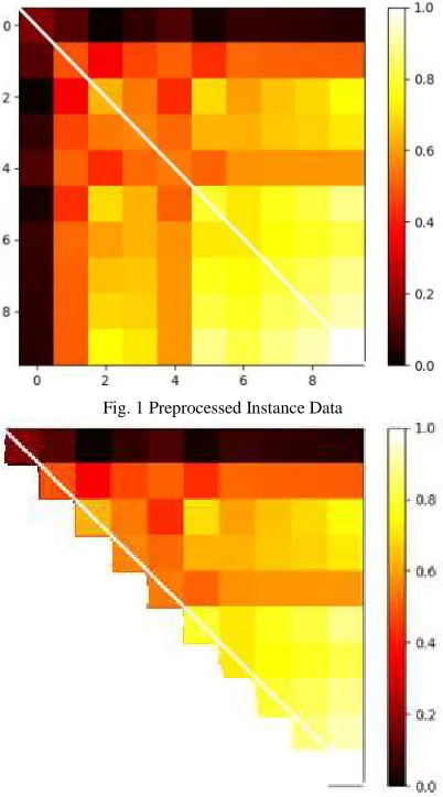
As mentioned before, the purpose of this preprocessing technique is for transforming an instance data with less information (small attributes) to an instance data with more information (large attributes). The result of this process is a 2D-shape instance data with the size of j x j (as much as the number of generated dummies) or i x i (as much as the number of input attributes) depend on which equation that is used (equation 5 or 6). Illustration of an instance that is preprocessed by using our proposed feature extraction technique is shown in Figure 1.

Since it is a covariance matrix, the pixel value above the main diagonal is always the same with the pixel under the main diagonal (white line, see Figure 1). In other words, this can be said to be symmetrical. Thus, we can prune the pixel data under the main diagonal to prevent redundancy and speed up computation time in the next process. This step is called pixel pruning and the total number of pixel data after pruning is always satisfying equation 8 [12].

Fig. 1 Preprocessed Instance Data

Fig. 2 Preprocessed Instance Data (with pixel pruning)

5 =

Where p is the number of pixel data after the pruning process (data above diagonal and pixel in diagonal) and s is the side length of the matrix. Illustration of preprocessed instance data after the pruning process can be seen in Figure 2.

The entire process of the proposed feature extraction algorithm can be summarized as follows:

• Load dataset and count number of instances and input attributes.

• Calculate the average and standard deviation of each input attributes.

• Calculate the probability density of each instance in each attribute.

• Generate j dummy instances based on the Gaussian distribution function.

• Normalize all generated dummy instance by using min-max scalar.

• Do matrix multiplication for each dummy matrix with their transpose matrix to obtain the covariance matrix for each instance.

• Do final normalization for each pixel data in covariance matrix using min-max scalar.

• Do pixel pruning to trim redundant data.

• Reshape or flatten the data in each instance before the processing step (modeling with ML algorithm).

D. Performance Measurement and Comparison

As mentioned before, a machine learning (ML) algorithm, optimization, and validation technique are used to model data and measure the performance of using the selected feature extraction algorithm. In this research, a simple ML algorithm called k-nearest neighbor (KNN) [13] is used to model the data and also test the effectiveness of the proposed feature extraction algorithm. Then, an optimization method called grid search [14] is applied to find the best number of k in KNN in which getting the highest accuracy in the data processing. The grid search algorithm will find the best number of k in the range of 1 to 50 with the step of 1. To obtain the value of accuracy itself, a validation mechanism called K-fold

TABLEIVV

NUMBER OF MISSING VALUE AND IMPUTATION VALUE

Class

Actual Class State (1) State (0)

Predicted Class

State (1) True Positive (TP) False Positive (FP)

State (0) False Negative (FN)

True Negative (TN)

Accuracy =_<=6<>6?=6?><=6<> (9)

Where TP is true positive which shows the number of correct prediction of class 1, TN is true negative which shows the number of correct prediction of class 0, FP is false positive which shows the number of false prediction of class 1, and FN is false negative which shows the number of false prediction of class 0. The illustration of TP, TN, FP, and FN can be seen by the confusion matrix in Table 4 [16].

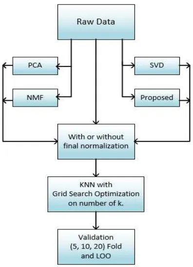
Finally, to see how good our proposed technique is, we also perform a comparison with another feature extraction algorithm which are principal component analysis (PCA) [17], non-negative matrix factorization (NMF) [18], singular value decomposition (SVD) [19][20], and with raw data processing. The process diagram of this experiment is shown in Figure 3. Different from PCA, NMF, and SVD which can only extract new attributes as much as the number of input attributes maximally, our proposed algorithm is able to extract new attributes as much as the square of the number of generated dummies. The number of generated dummies can be tuned until it meets the limit of computing power because the larger attributes will cause high computational cost.

III. RESULTS AND DISCUSSION

In this chapter, we describe the performance comparison result of our proposed algorithm against the other feature extraction algorithms. The parameter that is used to justify the performance of the model is accuracy. Accuracy defines how good a model in predicting the class (pond state) of given data. The higher the accuracy, the better the model.

Fig. 3 Process diagram of data processing

As shown in Figure 3, there are 4 kinds of validation to measure the performance of each model. The model is developed using optimized KNN algorithm (KNN + grid

search) which processes the supervised data (aquaculture dataset) with the help of certain data preprocessing technique. In this test, we take several accuracy values from several numbers of dummies for our algorithm and several numbers of components for other feature extraction algorithms. Then we take the best one to be compared with the others.

A. 5-Fold Cross-Validation

In 5-fold CV, the data is divided into 5 parts. At the first iteration, the first part becomes the test data, and the rest become the train data. Train data is a set of data which is used by an optimized KNN algorithm to develop a model. Test data is a set of data which is used to test the model and measure its performance. In the next iteration, the second part becomes the test data, and the rest become the train data. This scenario is repeated until each part has become train data and test data. Thus, there are 5 values of accuracy and the final accuracy result is obtained by averaging.

The comparison result of the proposed technique against raw data processing and other feature extraction algorithms can be seen in Figure 4.

Fig. 4 Comparison Result in 5-Fold CV

Fig. 5 Comparison Result in 10-Fold CV

As shown in Figure 4, both of our proposed algorithms give the best performance compared to the others. Proposed 1 stands for our proposed algorithm without pixel pruning while the proposed 2 is improved with pixel pruning. Both accuracies is 0.707 and 0.707, respectively.

B. 10-Fold Cross-Validation

In 10-fold CV, the data is divided into 10 parts, and the rest process is the same as the previous test. Thus, there are 10 values of accuracy, and the final result is calculated by

0,678 0,661

0,701 0,701 0,707 0,707

0,6 0,65 0,7 0,75

Raw(k:29)+z PCA (k:22, n:5)+z NMF (k:45, n:13) SVD (k:50, n:10)+z Proposed 1 (k:7, j:30)+z Proposed 2 (k:7, j:30)+z

5- fold Accuracy

0,69

0,701 0,701 0,701 0,701 0,701

0,68 0,69 0,7 0,71

Raw(k:31)+z PCA (k:6, n:5)+z NMF (k:30, n:10)+z SVD (k:42, n:10)+z Proposed 1 (k:9, j:30)+z Proposed 2 (k:9, j:30)+z

averaging all accuracy values. The comparison result of the proposed technique against raw data processing and other feature extraction algorithms can be seen in Figure 5. All of the feature extraction algorithms are giving the same best result compared to raw data processing which is 0.701.

C. 20-Fold Cross-Validation

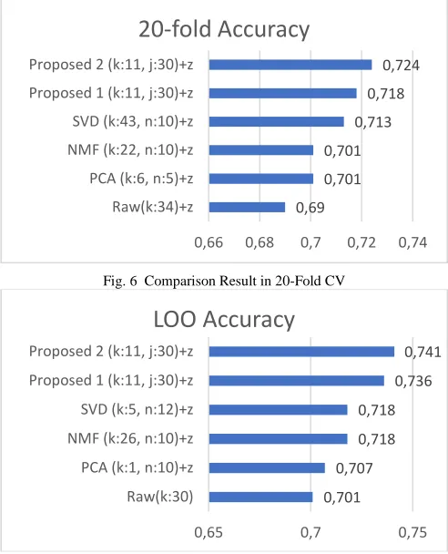
In 20-fold CV, the data is divided into 20 parts, and the process is the same as the scenario of the previous test. Thus, there are 20 values of accuracy, and the final result is calculated by averaging all of them. The comparison result of the proposed technique against raw data processing and other feature extraction algorithms can be seen in Figure 6. Our proposed algorithms are giving the best result compared to the other feature extraction algorithms. The accuracy of both proposed algorithms (1 and 2) are 0.718 and 0.724, respectively.

D. Leave One Out Validation

In LOO validation, the data is divided into as much as the number of instance in the dataset. In this research, we use aquaculture data which contains 174 instance data. Therefore,

Fig. 6 Comparison Result in 20-Fold CV

Fig. 7 Comparison Result in LOO Validation

by using LOO validation, there are 174 parts of data with only 1 instance in each part. The rest process is the same as the previous scenario. In other words, 1 instance becomes the test data and the rest become train data. Then, the process is repeated until each instance has become either train data or test data. LOO validation takes more computation time since it divides and processes the data into as much as the number of instances. Thus, there are 174 values of accuracy, and the final result is calculated by averaging all of them. The comparison result of the proposed

technique against raw data processing, and another algorithm can be seen in Figure 7. Our proposed algorithms are giving the best result compared to the others. The accuracy of both proposed algorithms (1 and 2) are 0.736 and 0.741, respectively. All of the experiment results of this research can be seen in Appendix 1b.

IV. CONCLUSIONS

As a result of the previous chapter, we can conclude that the higher accuracy can be achieved by using any feature extraction algorithms. Both of our proposed algorithms are giving the best performance in all kind of validation. In 10-fold validation, the algorithms give the best performance as good as the other feature extraction techniques with the accuracy value of 0.701 and surpass the raw data processing. However, the proposed 2 algorithms (with pixel pruning) is exceeding PCA, NMF, SVD, and raw processing in 5-fold, 20-fold, and LOO validation with the accuracy value of 0.707, 0.724, and 0.741 respectively. Besides that, the runner up is still held by our proposed 1 algorithm (without pixel pruning) where the accuracy value is 0.707, 0.718, and 0.736 respectively. Compared in all kind of validation, the accuracy of the proposed method with pixel pruning is better than the proposed method without pixel pruning. This is happening because data redundancy is prevented in pixel pruning. It also makes the computation time faster since it computes fewer pixel attributes. Then, as shown in appendix 1a, the global top 5 accuracies is achieved all by our proposed method which proves that it is the best solution for the task in the dataset.

Our proposed method indeed has given the best performance but may still not optimal yet. The best accuracy when it is combined with KNN and grid search algorithm is just 0.741. For the future work, we will perform further study about ML and optimization algorithm to achieve higher accuracy. There are plenty of algorithms that can be compared like support vector machine (SVM), decision tree, genetic algorithm (GA), particle swarm optimization (PSO), etc. But, since it has large attributes to be computed and formed 2D-shape data, a deep learning algorithm especially convolutional neural networks (CNN) may be the solution to achieve maximum accuracy. A further study about CNN/ConvNet, hyper-parameters tuning and any kinds of its architectures such as LeNet, VGGNet, ResNet, Inception, etc will be studied in the next research. Finally, the developed model will be used as the knowledge domain for a decision support system in giving aquaculture recommendation.

NOMENCLATURE

The following nomenclature is used for abbreviation in Figure 4 to 7.

k : the best number of k in KNN based on grid search optimization.

j : number of j dummies of proposed algorithm n : number of n components of PCA or NMF or SVD +z : with final normalization (see equation 7)

0,69 0,701 0,701

0,713 0,718

0,724

0,66 0,68 0,7 0,72 0,74

Raw(k:34)+z PCA (k:6, n:5)+z NMF (k:22, n:10)+z SVD (k:43, n:10)+z Proposed 1 (k:11, j:30)+z Proposed 2 (k:11, j:30)+z

20-fold Accuracy

0,701 0,707

0,718 0,718

0,736 0,741

0,65 0,7 0,75

Raw(k:30) PCA (k:1, n:10)+z NMF (k:26, n:10)+z SVD (k:5, n:12)+z Proposed 1 (k:11, j:30)+z Proposed 2 (k:11, j:30)+z

ACKNOWLEDGMENT

We would like to thank Mr. Junaedi Ispianto for supporting the aquaculture dataset which is used in this research as a study problem.

REFERENCES

[1] Ruslisan, N. H. Kalam, A. C. Dwininta, M. H. Habibi, E. T. Rahayu, N. Dewi, E. E. Henny, and W. Widyatmanti, “Water quality assessment using remote sensing and GIS for in-shore marine environment suitability,” Aquacultura Indonesiana, vol. 17, pp. 46-53, 2016.

[2] D. Yuswantoro, O. Natan, A. N. Angga, A. I. Gunawan, Taufiqurrahman, B. S. B. Dewantara, A. Kurniawan, “Fuzzy logic-based control system for dissolved oxygen control on indoor shrimp cultivation,” in Proc. International Electronics Symposium on

Engineering Technology and Applications (IES-ETA), 2018, p. 37.

[3] M. Muslim, M. Fitrani, and A. M. Afrianto, “The effect of water temperature on incubation period, hatching rate, normalities of the larvae and survival rate of snakehead fish channa striata,” Aquacultura Indonesiana, vol. 19, pp. 90-94, 2018.

[4] Djumanto, Ustadi, Rustadi, and B. Triyatno, “Utilization of Wastewater from Vannamei Shrimp Pond for Rearing Milkfish in Keburuhan Coast Purworejo Sub-District,” Aquacultura Indonesiana, vol. 19 (1), pp. 38-46, 2018.

[5] D. Ayon, “Machine Learning Algorithms: A Review,” International

Journal of Computer Science and Information Technologies, vol. 7

(3), pp. 1174-1179, 2016.

[6] M. Khadr and M. Elshemy, “Data-driven modeling for water quality prediction case study: The drains system associated with Manzala Lake, Egypt,” Ain Shams Engineering Journal, vol. 8, pp. 549-557, 2016.

[7] L. Xu and S. Liu, “Study of short-term water quality prediction model based on wavelet neural network,” Mathematical and

Computer Modelling, vol. 58, pp. 807–813, 2013.

[8] G. Tan, J. Yan, C. Gao, and S. Yang, “Prediction of water quality time series data based on least squares support vector machine,” in

Proc. International Conference on Advances in Computational Modeling and Simulation, 2012, p. 1194.

[9] C. Deng, Y. Gao, J. Gu, X. Miao, and S. Li, “Research on the growth model of aquaculture organisms based on neural network expert system,” in Proc. 6th _{International Conference on Natural}

Computation, 2010, p. 1812.

[10] I. Ahmad, M. Basheri, M. J. Iqbal and A. Rahim, “Performance Comparison of Support Vector Machine, Random Forest, and Extreme Learning Machine for Intrusion Detection,” IEEE Access, vol. 6, pp. 33789-33795, 2018.

[11] D. Banik, A. Ekbal and P. Bhattacharyya, “Machine Learning Based Optimized Pruning Approach for Decoding in Statistical Machine Translation,” IEEE Access, vol. 7, pp. 1736-1751, 2019.

[12] B.S.B. Dewantara and J. Miura, "Estimating Head Orientation using a Combination of Multiple Cues", IEICE Trans. on Information and

Systems, vol. E99-D, no. 6, pp. 1603-1613, 2016.

[13] F. Zhao and Q. Tang, “A KNN Learning Algorithm for Collusion-Resistant Spectrum Auction in Small Cell Networks,” IEEE Access, vol. 6, pp. 45796-45803, 2018.

[14] A. Rojas-Domínguez, L. C. Padierna, J. M. Carpio Valadez, H. J. Puga-Soberanes and H. J. Fraire, “Optimal Hyper-Parameter Tuning of SVM Classifiers With Application to Medical Diagnosis,” IEEE

Access, vol. 6, pp. 7164-7176, 2018.

[15] J. Tong, J. Xi, Q. Guo and Y. Yu, “Low-complexity cross-validation design of a linear estimator,” Electronics Letters, vol. 53, no. 18, pp. 1252-1254, 2017.

[16] D. M. W. Powers, “Evaluation: From Precision, Recall and F-Measure to ROC, Informedness, Markedness & Correlation,”

Journal of Machine Learning Technologies, vol. 2, no. 1, pp. 37–63,

2011.

[17] B. N. Li, Q. Yu, R. Wang, K. Xiang, M. Wang and X. Li, “Block Principal Component Analysis With Nongreedy L1-Norm Maximization,” IEEE Transactions on Cybernetics, vol. 46, no. 11, pp. 2543-2547, 2016.

[18] M. Šavc, V. Glaser, J. Kranjec, I. Cikajlo, Z. Matjač_ič _{and A.} Holobar, “Comparison of Convolutive Kernel Compensation and Non-Negative Matrix Factorization of Surface Electromyograms,”

IEEE Transactions on Neural Systems and Rehabilitation Engineering, vol. 26, no. 10, pp. 1935-1944, 2018.

[19] N. Halko, P. G. Martinsson, and J. A. Tropp, “Finding structure with randomness: Stochastic algorithms for constructing approximate matrix decompositions,” Society for Industrial and Applied

Mathematics, vol. 53, pp. 217-288, 2011.

APPENDIX

Appendix 1: Table of Accuracy Comparison in All Scenarios

a. Summary:

Table of Global Top 5 in Accuracy Comparison

Global Top 5 Notes

Accuracy Method

0.741 Proposed 30x30 -> final normalization -> pixel pruning (LOO)

0.736 Proposed 30x30 -> final normalization (LOO)

0.73 Proposed 50x50 -> pixel pruning (LOO)

0.724 Proposed 50x50 (LOO)

0.724 Proposed 30x30 -> final normalization -> pixel pruning (20-fold)

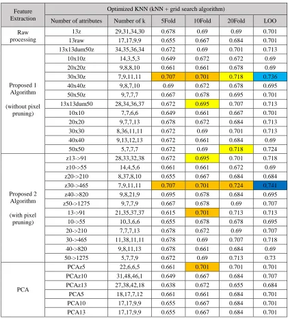
b. Comparison Table: (See appendix 1c for nomenclature)

Table of Accuracy Comparison in All Scenario

Feature Extraction

Optimized KNN (kNN + grid search algorithm)

Number of attributes Number of k 5Fold 10Fold 20Fold LOO Raw

processing

13z 29,31,34,30 0.678 0.69 0.69 0.701 13raw 17,17,9,9 0.655 0.667 0.684 0.701

Proposed 1 Algorithm (without pixel

pruning)

13x13dum50z 34,35,36,34 0.672 0.69 0.701 0.713 10x10z 14,3,5,3 0.649 0.672 0.672 0.69 20x20z 9,8,8,10 0.661 0.661 0.678 0.69 30x30z 7,9,11,11 0.707 0.701 0.718 0.736 40x40z 9,8,7,10 0.69 0.672 0.678 0.695 50x50z 9,7,7,7 0.667 0.678 0.695 0.701 13x13dum50 28,34,36,37 0.672 0.695 0.707 0.713 10x10 7,7,6,6 0.649 0.661 0.667 0.701 20x20 9,7,7,13 0.678 0.672 0.684 0.713 30x30 8,36,11,11 0.672 0.69 0.701 0.713 40x40 9,13,12,13 0.672 0.661 0.684 0.69 50x50 5,7,7,7 0.672 0.69 0.718 0.724

Proposed 2 Algorithm (with pixel pruning)

z13->91 28,33,32,38 0.672 0.695 0.701 0.718 z10->55 14,4,5,6 0.661 0.661 0.672 0.69 z20->210 8,37,8,10 0.655 0.667 0.684 0.684 z30->465 7,9,11,11 0.707 0.701 0.724 0.741 z40->820 9,8,21,9 0.695 0.678 0.684 0.695 z50->1275 9,7,7,9 0.667 0.678 0.69 0.707 13->91 21,35,37,37 0.615 0.701 0.713 0.713 10->55 10,3,6,6 0.655 0.678 0.678 0.695 20->210 7,7,7,13 0.678 0.672 0.69 0.707 30->465 11,38,11,11 0.678 0.69 0.707 0.718 40->820 9,8,11,13 0.678 0.661 0.684 0.69 50->1275 5,7,7,9 0.672 0.69 0.713 0.73

PCA

NMF

NMFz5 25,19,13,24 0.661 0.655 0.678 0.69 NMFz10 28,30,22,26 0.684 0.701 0.701 0.718 NMFz13 19,32,39,20 0.667 0.695 0.678 0.672 NMF5 14,18,18,5 0.667 0.678 0.678 0.684 NMF10 45,49,5,5 0.672 0.638 0.638 0.672 NMF13 45,28,10,12 0.701 0.586 0.672 0.621

SVD

SVDz5 27,24,38,1 0.649 0.672 0.69 0.69 SVDz10 50,42,43,5 0.701 0.701 0.713 0.713 SVDz12 36,44,39,5 0.69 0.695 0.695 0.718 SVD5 18,17,9,9 0.661 0.678 0.69 0.701 SVD10 17,17,9,9 0.655 0.667 0.684 0.701 SVD12 17,17,17,9 0.655 0.667 0.655 0.701

c. Notes:

13raw : raw data (13 input attributes).

13z : same as above but with min-max normalization.

10x10 : in the proposed algorithm, it is made 10 dummy instances, then it follows the equation 5 in calculating the covariance matrix, so it has the number of attributes of 10x10 = 100 pixels. 10x10z : same as above but with final normalization (see equation 7) in the last step.

13x13dum50 : in the proposed algorithm, it is made 50 dummy instances, then it follows the equation 6 in calculating the covariance matrix, so it has the number of attributes of 13x13 = 169 pixels. 13x13dum50z : same as above but with final normalization (see equation 7) in the last step.

10->55 : pixel pruning from 10x10, (see equation 8).

z10->55 : same as above but with final normalization (see equation 7).

PCA5/NMF5/SVD5: other feature extraction algorithms (PCA, NMF, and SVD) with 5 components. PCAz5/etc… : same as above but with min-max normalization.