A New Nonlinear Specification of Structural Breaks for Money Demand in Iran
Esmaiel Abounoori Department of Economics,
Semnan University, Semnan-Iran.
Behnam Shahriyar
Department of Economics & Management, Fazilat Higher Education Institute,
Semnan-Iran. [email protected]
Abstract
In a structural time seriesregression model, binary variables have been used to quantify qualitative or categorical quantitative events such as politic and economic structural breaks, regions, age groups and etc. The use of the binary dummy variables is not reasonable because the effect of an event decreases (increases) gradually over time not at once. The simple and basic idea in this paper is to involve a new transition function in a structural time series regression equation model in order to transform the binary dummy variables into a fuzzy set. The main purpose of this paper is to present a new method for endogenous modeling structural breaks in money demand function using fuzzy set. Hence, we model structural breaks in a money demand function via fuzzy set theory, transition functions and binary dummy variables and compare these. After introducing a new transition function, we model money volume shock in 1992 in money demand function. The results indicate that our transition function has better characteristics and accurate results than the binary dummy variable, exponential and logistic transition functions.
Keywords: Dummy Variable, Fuzzy Set, Structural Break, AS Membership Function, Money Demand, Iran.
JEL Classification: C10, C52
1. Introduction
According to the econometrics literature, the dummy variables are used to quantify the qualitative events and/or the structural breaks. The dummy variable is equal to 0 and 1 when an event is not present and during in which is present, respectively. Because of structural breaks, parameters of empirical economic equations are changed over time. Accordingly, Perron (1989) introduced unit root with structural breakpoint test and presented that the main reason of economic time series non stationarity is occurrence of qualitative shocks and events (Perron, 1989). It seems that we should define effects of qualitative shocks and events according to stationarity and non- stationarity of time series.
The application of the binary dummy variable is based on a relatively unrealistic assumption: according to the binary dummy variable either the effect of a qualitative variable exist (D=1) or the effect does not exist (D=0). In reality the effect may start at once, but in general depreciates (appreciates) gradually within a period of time. Thus, it is more reasonable to introduce a dummy variable as a fuzzy set. The decreasing (increasing) period may be short or long. A dummy variable as a fuzzy set can better reflect the gradual reduction of the effect.
Consequently, linear models with binary dummy variables have misspecification, while, nonlinear models (intrinsically linear or nonlinear) with fuzzy dummy variables can have better specifications than linear models.
Therefore, the main problem of this paper is that effect of qualitative events on dependent variable increases, decreases or constant over time. Consequently, we can say that if dependent variable is stationary then effect of qualitative shock or event decrease over time.
In this work we propose a different approach to arrive at the demand for money in Iran. We assume that M1 reflects to a greater extent the
money volume shocks (Granger & Teräsvirta, 1993; Teräsvirta, 1994). In this paper, we can show that the demand for money in Iran can be represented by a, noninvertible, a new nonlinear specification of the STR type as well as logistic STR (LSTR). Moreover, our nonlinear representation is consistent with the theory. Findings of nonlinearities in money demand functions are gaining in evidence overtime.
This paper includes 5 sections; Second section includes a theoretical discussion of the fuzzy sets and structural breaks as a fuzzy variable, then we present a new approach to calculate membership function of this variable. Third section is devoted to the data analysis (this is the same as transition function in STR model). Empirical results are provided in section 4. The paper ends with summery and conclusion in section 5, with also appendices.
2. Theoretical Discussion
Before 1960s, classical mathematic theory was dominant in theoretic and applied mathematics. In this decade, theory of fuzzy was presented by Professor Lotfi Zadeh. He presented fuzzy sets, fuzzy algorithm, concept and application of linguistic variables in 1965, 1968 and 1978, respectively. Then, Black (1973) presented logical analysis and membership functions in his paper. Tanaka et. al (1982) introduced fuzzy regression and used linear programming for estimating fuzzy regression parameters.
Baliamoune (2000) applied a logistic member function for dummy variables, indirectly.
Giovanis (2009) applied fuzzy dummy variables with triangular membership function for studying effect of good or bad days on stock return. He takes in to triangle member ship functions for these variables. In this paper, by fuzzification of binary dummy fuzzy variables, Giovanis showed that fuzzy dummy variables how better results than (classical) dummy fuzzy variables, so that classification 0, 1 for days is week.
Bolotin (2004) used fuzzy dummy variable for fuzzifying Indicator Variables in Linear Regression Models in Medical Decision Making.
Abounouri and Shahriyar (2014), have used IIRF fuzzy dummy variables in order to modelling of Lucas Critique. They have estimated two models; one supply function model in Iran, and the other money demand function of Iran. Abounouri and Shahriyar (2013), have used Fuzzy approach to model the nonlinear structural breaks concerning money demand function in Iran. The main purpose of this paper is to compare LSTAR and ESTAR models with proposed model by Abounouri and Shahriyar (2013) (AS) concerning the money demand function of Iran.
Application of the Binary Dummy (BD) variable is based on a relatively unrealistic assumption: according to the Binary Dummy variable either the effect of a qualitative variable exist (D=1) or the effect does not exist (D=0). In reality the effect may start at once, but in general depreciate gradually within a period of time. Thus it is more reasonable to introduce a dummy variable as a Fuzzy set.
In the classical mathematics, a quantity is either a member of a set or isn’t. In other words, if Y is a reference set,
A
is a subset of Y (AY) and if x is a member of Y, we can write:(1)
A
1, x A
X (x)
0, x A
In whichXA (x) is the characteristic function. If
x
A
, then 1
(x)
XA and if
x
A
, thenXA (x)0. In fuzzy mathematics, (x)XA is changed to
A(x) that is a membership function of x [5]. Therefore, we have:1, is perfect member of A
( ) (0,1), is imperfect member of A (2)
0, A
x
x x
x A
) (x
A
is a membership function and the membership degree ofA
is important. In a classical linear regression model using Binary Dummy variable (BD), we can write:t t t t
Y
X
BD u(3)
t A
1, t A
BD X (t)
0, t A
Where t is the time (trend) variable that means,
0 ,
( ) , {0,1}
( ) ,
t s
t t
t s e
X t t
E Y DB
X t t t
2.1 Determination of fuzzy membership function
In fuzzy mathematics, fuzzification of a set is determined by constructing membership function or degrees (Sivanandam, Sumathi, & Deepa, 2007). Determination of membership function or degrees depends on their application. Fussiness in a set is characterized by determining its membership function. This classifies the elements in the set, whether they are discrete or continuous. Definition of a fuzzy set is completed by determining membership function according to its application. The shape of the membership function is an important criterion. Because if membership function is not characterized correctly (based on stationarity or non-statioarity), then all studies and analysis will deviate, so that regression model will have misspecification.
As Giovanis (2009) and Bolotin (2004), on the contrary with other researches where the dependent variable is fuzzy and so we have fuzzy interval estimations, our analysis is based to the fuzzification of the dummy variables representing the shock effects to show the weakness of the classification of one and zero dummy variables which leads to is classification errors. Here, dependent variable can be crisp. In fact, fuzzification consists in to change crisp variable (classical) to a fuzzy set. For this, we have to define the fuzzy rules.
For deriving fuzzy degrees, we can use intuition, inference, neural network and etc methods (Selmins, 1987). But, here, we use our transition function (AS), logistic and exponential transition functions (which were introduced by Granger and Träsvirta (1994) and Träsvirta (1994)) for modeling effect of a structural break in money demand function (Abounouri & Shahriyar 2013 & 2014).
Fuzzy Dummy (FD)variable in which the binary set,
0,1 , will be changed to the fuzzy membership function[0,1]:) 4 ( , 0 , ) ( 0 , 0 ) (
t t t t t dt t f t t t FD e e s S A t
If we suppose that the effect of the shock decreases gradually over time, we can write:
) 5 ( 0 ) ( dt DF d
So that, we can introduce a differential equation in the rectangular ABCD as follows:
) 6 ( ) ( ) ( t f dt DF d
Assumingts 0, the differential equation would be:
) 7 ( 0 , ) ( )
( 1
e e t t t dt FD d
In which
is the intensity parameter of the shock that has 3 forms:) 8 ( 1 1 1 0 ) ( ) 1 ( ) ( 0 2 ) ( 2 0 2 ) ( 2 0 2 ) ( 2 2 2 2 2 dt DF d dt DF d dt DF d e e t t t dt FD d
General solution of equation (9) is as follows:
) 9 ( 0 , ) ( ) ( ) ( 1
e e e t t c FD dt t t t FD d) 10 ( 0 , ) (
1
e
t t FD
The parameter
has to be determined within regression model. In fact, we select a
, which can minimize error sum of squares. Consequently, we can include the following FD function into a classical linear regression. ) 11 ( , 0 , ) ( 1 0 , 0 ) ( t t t t t t t t t t t t FD s e s s e s s A t )
12
(
t t tt
X
FD
u
Y
Here after we call this function “AS” fuzzy membership or transition function.
Equation (12) is a nonlinear regression equation with parameters, , and
to be estimated;[0,),
0 means that there has been no shock at all; If
1, the effect of shock will reduce decreasingly. If1
, effect of shock will reduce increasingly and if
1, equation (16) changes to a linear form and if
tend to infinity ( ) then the FD will be transformed to the BD.In nonlinear equation (12), the parameters
andas well as
and can be estimated by Nonlinear Least Squares (NLS). In other words, we can estimate the parameters including
, which minimizes Residual Sum of Squares (RSS). Consequently, we will find highest significant relation between ( s )e
t
t and the dependent variable. The start of the shock is either observable due to date happened and/or can be found by the break point of the Chow test. An important point in FDt is to select end time of
the shock effect( )te . A suggested method is to use a response function of
t
Y.
) 13 ( 0 , 0 , ) ( 0 , 0 ) ( 0 t t t t t t t t t t t t FD e e s e l s A t
A nonlinear parametric alternative model is Smooth Transition Regression (STR) model which introduced Granger and Träsvirta (1994) and Träsvirta (1994). In this model, the transition function can be parameterized either as a logistic function, in whose case we have a logistic STR (LSTR) model:
, ,
1 exp
, 0 (14) 1 1
K k k t tt G C S S C
FD
or as an exponential function, in whose case we have an exponential STR (ESTR) model:
, ,
1 exp
, 0 (15) 1
K k k t tt G C S S C
FD
Generally K 1 or K 2are selected.
3. Money Demand Model Specification
In this paper, we have used money demand data to compare the application of BD, ASTR (AS Transition Function), ESTR and LSTR model.
We use quarterly time series of national real money demand (M), national real GDP (G), nominal interest rate (i), GDP deflator Inflation (Inf) and exchange rate of US $ in Iran, from 1990:2 to 2008:3 (all variables are in constant price of 1997). The data is obtained from Central Bank of Iran. Based on these data, we estimate money demand function for Iran, and study effect of oil production shock (in 1992) on this function. In this year, because of increase in oil production and government revenue of oil sales, money volume increased function (Abounouri & Shahriyar 2013 & 2014).
In this paper, money demand function is specified as follows:
)
16
(
inf) ( 0 3 21
ie
ER
G
M
) 17 ( inf) ( 3 2 1
0
LnG LnER i
LnM
Here we use M1 definition for money volume.
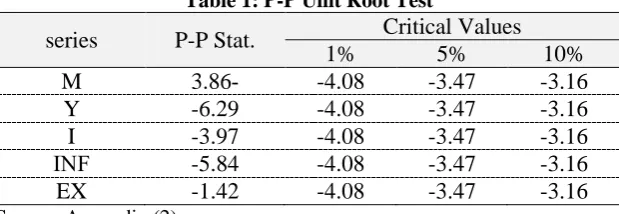
According to the Chow test in appendix (1), the start point of monetary policy shock is observed on 1992:3. Due to the structural break, we have used Philips-Peron unit root test. According to the results in appendix (2) summarized in table (1), all variables except EX are stationary.
Table 1: P-P Unit Root Test
series P-P Stat. Critical Values
1% 5% 10%
M 3.86- -4.08 -3.47 -3.16 Y -6.29 -4.08 -3.47 -3.16 I -3.97 -4.08 -3.47 -3.16 FNI -5.84 -4.08 -3.47 -3.16 EX -1.42 -4.08 -3.47 -3.16
Source: Appendix (2)
4. Empirical Results
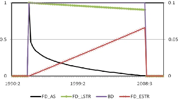
The nonlinear approach over the BD variable has been justified concerning the following practical evidences. Ln(M) is regressed on Ln(G(-1)), I-INF and Ln(EX(-2)) including binary dummy variable and fuzzy (nonlinear) dummy variables. The estimation and prediction results of models are shown in Table (2). FD is the membership function, and estimated as follow:
) 18 ( )] (0.003 [1 _ ) 001 . 0 ( _ ) 75 ( 1 _ 1 -15 . 0 t Exp ESTR FD t Exp ESTR FD t AS FD
FD=0, before 1992:3. According to the estimated results
0.15 shows nonlinearity of money demand.rational than the others, consequently shock effect on money demand depreciate more rapid.
Figure 1: Graphs of the Membership Functions
Table 2: Estimation and Prediction Results
Model\ Variable
Co
n
sta
n
t
Ln
(G(
-1
))
I-INF
Ln
(EX(
-2
))
Bin
ary
Du
m
m
y
Va
riab
le / R
2
Ad
.R
2 F
D.W RM
S
E
Binary 1.97 -0.37 -0.29 0.07 -0.28 - 0.62 0.60 27.30 1.84 53.76 (0.48) (0.05) (0.44) (0.03) (0.04)
ESTR 5.42 0.17 0.19 -0.13 - -0.001 0.58 0.56 23.30 0.91 56.41 (1.15) (0.09) (0.55) (0.04) (0.0001)
LSTR 10.80 0.17 0.18 -0.13 - 0.002 0.58 0.56 23.20 0.90 56.51 (2.32) (0.09) (0.55) (0.05) (0.0004)
ASTR 0.46 0.47 -0.63 0.15 - 0.15 0.69 0.68 38.30 2.06 50.39 (0.08) (0.04) (0.44) (0.06) (0.05)
Sources: Appendices (3) and (4)
which are based on the Binary dummy variable, ESTR and LSTR. We can conclude that ASTR Model has less measuring error (misspecification error) than the others. Moreover, based on prediction of M, ASTR model has clearly less MSE than the other models; prediction results are shown in appendix (4).
All coefficients of ASTR model except real interest rate are significant in %5 probability level. Real interest rate is significant in %16 probability level. This variable isn’t significant in the other models. Whereas according to D.W. statistics in table (2), in spite of ASTR and Binary models, ESTR and LSTR models have autocorrelation problem. According to theories of demand for money such as transactions demand for money and speculative demand for money, elasticity of money to GDP and real interest rate should be positive and negative, respectively. Whereas if elasticity of money to exchange rate is to be significant, there will be money substitution phenomena. These theories are confirmed only in ASTR model. For example, despite of transactions theory of demand for money in binary model, effect of GDP on demand for money is negative.
Not that intensity parameter
is less than 1 in ASTR model, this mean that effect of structural break (as a result of money supply shock) has been depreciated overtime. This result is more applicable to stationarity and Philips-Perron unit root test.5. Summery and Conclusion
A significant part of the empirical researches has been devoted to the search for robust econometric specifications of empirical models of the demand for money with the desired property of theoretical coherence.
For modeling structural breaks in money demand function, we proposed a new Smooth Transition Regression (STR) which is named ASTR under fuzzy set theory. The idea in this paper has been to use the smooth parametric transition function as well as the logistic transition function has been presented by Granger and Teräsvirta (1994), F(t) = 1-[(t– ts)/ (te – ts)]λ , to model endogenously a shock (structural
break) in demand for money time series. Characteristics of this transition function are flexible because at time ts there is an interruption in the
series, that is, an impulse shock, that fully dissipates by time te. The
function F(t) is everywhere zero except in the interval (ts,te], with the
λ→0, and F(t) → 1 as λ→ ∞. Thus, the shock is most persistent when λ is large. In fact, when F(t) = 1, using the parametric function is equivalent to using a single binary dummy variable in the interval (ts, te].
Therefore, we have introduced a fuzzy dummy variable (AS transition function) alternative to that of the hard binary dummy variable, exponential and logistic transition functions.
As mentioned above, for purposes of this paper, we estimate money demand function of Iran and modeled structural break in 1992:3 by ASTR, Binary Dummy Variable, ESTR and LSTR models. The main results of this paper can be as follows:
It is important that researches take into dummy variables as fuzzy sets, because measurement of these is ambiguous.
ASTR model has more mathematical flexible characteristics and better results in estimation and prediction. Consequently, ASTR model has less misspecification error than the other alternatives.
ASTR model structural breaks endogenously and involve stationarity and non-stationarity of dependent variable time series. In other word, we can say that if dependent variable is stationary then effect of shock decrease over time then parameters of regression return to before of the shock overtime (parameters are time varying). This property was observed in money demand function estimated for Iran in this paper.
Acknowledgment
We would like to thank the editorial board as well as unanimous referees of the Journal whose comments have been helpful improving this paper.
References
Abounouri, E. & Shahriyar, B. (2013). Modelling of Lucas Critique using Fuzzy Set Approach. Journal of Economic Research, Tehran University, 49(2), 229-265.
Abounouri, E. & Shahriyar, B. (2014). Nonlinear Modelling of Structural Breaks concerning Money Demand Function in Iran using Fuzzy Approach. the Economic Research, Tarbiat Modares University, 13(4), 55-78.
Baliamoune, M. (2000). Economics of Summitry: an Empirical Assessment of the Economic Effect of Summits. 27, 295-314.
Bolotin, A. (2004). Replacing Indicator Variables by Fuzzy Membership Functions in Statistical Regression Models: Examples of Epidemiological Studies. Biological and Medical Data Analysis, 3337, 251 - 258.
Giovanis, E. (2009). Bootstrapping Fuzzy-GARCH Regressions on the Day of the Week Effect in Stock Returns: Applications in MATLAB. Working Paper.
Granger, C. J., & Teräsvirta, T. (1994). The Combination of Forecasts Using Changing Weights. International Journal of Forecasting , 10, 47-57.
Granger, C., & Teräsvirta, T. (1993). Modeling Nonlinear Economic Relationships. London: Oxford University Press.
Perron, P. (1989). The great crash, the oil price shock, and the unit root hypothesis. 57, 1361-1401.
Selmins, A. (1987). Least Squares Model Fitting To Fuzzy Vector Data. Fuzzy Sets and Systems, 8, 903-908.
Sivanandam, S., Sumathi, S., & Deepa, S. (2007). Introduction to Fuzzy Logic using MATLAB. New York: Springer.
Tanaka, H., Uejima, S., & Asai, K. (1982). Linear Regression Analysis With Fuzzy Model. IEEE Transactions on SMC, 12, 903-907.
Teräsvirta, T. (1994). Specification, Estimation and Evaluation of Smooth Transition Autoregressive Models. Journal of the American Statistical Association, 89, 208-218.
Teräsvirta, T. (1994). Testing Linearity and Modelling Nonlinear Time Series. Kybernetika, 30 (3), 319-330.
Zadeh, L. (1968). Fuzzy Algorithms. Information and Control, 12, 94– 102.
Zadeh, L. (1996). Fuzzy Logic = Computing with Words. IEEE Transactions on Fuzzy Systems, 4 (2), 103-111.
Zadeh, L. (1988). Fuzzy Logic. IEEE Computer Magazine , 21 (4), 177-186.
Zadeh, L. (1965). Fuzzy Sets. Information and Control, 8 (3), 338–353. Zadeh, L. (1978). Fuzzy Sets as a Basis for a Theory of Possibility. Fuzzy
Appendix: Computer base estimation results:
Appendix 1: Chow Breakpoint Test
Appendix 2: Philips-Perron test results
Appendix 3: Computer based estimation results
Appendix 4: Predictions results