An optimization-based algorithm for Coulomb's frictional contact

C. Besse, O. Goubet, T. Goudon & S. Nicaise, Editors

AN OPTIMIZATION-BASED ALGORITHM

FOR COULOMB’S FRICTIONAL CONTACT

Florent Cadoux

Abstract. The main goal of this paper is to propose a stable algorithm to compute friction forces governed by Coulomb’s law in the course of the simulation of a nonsmooth Lagrangian dynamical system. The problem appears in computational mechanics, to simulate the dynamics of granular materials, robots,etc. Using a classical impulse-velocity formulation of Coulomb’s law to model friction, and a semi-implicit time discretization scheme, we get a set of linear, non-linear and complementarity equations which has to be solved at each timestep. Two mutually dual parametric convex optimization problems coupled with a fixed point equation appear naturally. By solving (one of) these optimization problems iteratively within a damped nonsmooth-Newton algorithm, it is possible to decrease some infeasibility criterion and hopefully converge to a solution of the system. Numerical results are provided, which show that the number of iterations needed by the algorithm is very small in general and that the method is stable.

R´esum´e. Cet article propose un algorithme stable pour le calcul des forces de frottement r´egies par la loi de Coulomb lors de la simulation d’un syst`eme dynamique lagrangien non-r´egulier. Ce probl`eme apparaˆıt en m´ecanique num´erique, pour simuler la dynamique de mat´eriaux granulaires, robots,etc_.

En utilisant une formulation classique, dite impulsion-vitesse, de la loi de Coulomb pour mod´eliser le frottement, et un sch´ema de discr´etisation semi-implicite, on obtient un ensemble d’´equations lin´eaires, non-lin´eaires et de compl´ementarit´e, que l’on doit r´esoudre `a chaque pas de temps. Deux probl`emes d’optimisation convexes duaux l’un de l’autre, coupl´es `a une ´equation de point fixe, apparaissent naturellement. En r´esolvant l’un ou l’autre de ces probl`emes d’optimisation it´erativement dans un algorithme de Newton avec recherche lin´eaire, on peut diminuer un certain crit`ere d’infaisabilit´e avec l’espoir de converger vers une solution du syst`eme. Des r´esultats num´eriques sont fournis, qui montrent que le nombre d’it´erations n´ecessaires est tr`es petit en g´en´eral, et que la m´ethode est stable.

Introduction

The simulation of the dynamics of a mechanical system involving friction at contact points is an active area of research with a broad range of applications, from civil engineering [13] to robotics [4] and computer graphics [11]. It can be used to compute or control the motion, discuss equilibria, and even access information unavailable to experiments : for instance, the simulation of large systems of dry granular material provides insight on the repartition of forces in a pile of stones or sand grains.

In the first place, physical laws must be chosen to model friction (what is the force between two bodies which rub against each other ?) and impacts (what is the velocity of two bodies after an impact, knowing the velocities before the event ?). We advocate the use of Coulomb’s law of friction, described below in section 1, which is physically reasonable in many practical situations, along with a restitution coefficient to

1 _{Inria, 655 av. de l’Europe, 38334 Montbonnot}

c

EDP Sciences, SMAI 2009

model rebound. Many other approaches modify the problem by regularizing the friction law (this is often called Molecular Dynamics) [21] or by somehow linearizing it, typically using a polyhedral approximation of the second-order cone involved in Coulomb’s law [3]. By contrast, we use an exact impulse-velocity formulation (technique often referred to asContact Dynamics).

Different sources of nonsmoothness make the problem much more difficult, both theoretically and practically [6], than classical (that is to say, smooth) Lagrangian mechanics where the motion takes place on a manifold. When unilateral contact is involved, collisions can take place during which the motion of the dynamical system can change very quickly. For this reason, jumps must be expected in the velocities in general. In this paper, we focus on numerical aspects and simulation ; from this viewpoint, we deal with nonsmoothness as follows:

• unilateral constraints (two elements cannot penetrate each other) are enforced via the impulse-velocity formulation (section 1),

• friction forces governed by Coulomb’s law (a nonsmooth, multivalued law) are computed through an optimization-based algorithm, which is the main contribution of this paper,

• and jumps in velocities are handled by a time-stepping scheme (which, as opposed to event-driven schemes, does not consider every event, such as creation or disappearance of contact, separately). An overview of algorithms and numerical methods used in frictional contact Mechanics can be found in [7]. A well-known exact formulation of Coulomb’s law is the so-calledaugmented Lagrangian formulation, investigated by Alart-Curnier [1] (who solved the problem using a Newton-like algorithm, revisited in [8]), De Saxc´e-Feng [9] (who used a solver based on Uzawa’s algorithm) and Simo-Laursen [17]. Moreau [13,15], Jourdan-Alart-Jean [10] used a Gauss-Seidel like algorithm which solves the contact problem independently at each contact point, and then iterates until a global solution is found. In this paper, we propose a novel approach which handles all contacts globally and uses the structure of the problem to exhibit a natural optimization problem, namely a parametric second-order cone programming problem, coupled with a fixed point equation. The optimization problem can be solved iteratively until a solution to the fixed point problem, hence the contact problem, is found.

The paper is organized as follows. In section 1, we describe the physical meaning of Coulomb’s law for dry frictional contact, and the two classical ways to formulate it as a complementarity constraint, either between the gap and the force or between the impulse and the velocity. In section 2, we recall the equations of motion for a Lagrangian mechanical system with contact forces governed by the impulse-velocity formulation of Coulomb’s law, and we use a semi-implicit discretization scheme to derive a system of equations (the one-step problem) to be solved at each timestep. In section 3, we reformulate this sytem as a parametric optimization problem coupled with a fixed-point equation. The ability to practically solve and differentiate the parametric problem is finally used in section 4 in a damped nonsmooth Newton algorithm to minimize some infeasibility criterion, with the aim of converging to a solution of the one-step problem. Section 5 gathers some simple numerical experiments to assess the efficiency of the approach.

1.

Coulomb’s law of friction

Models used to describe friction depend on the nature of the materials in contact. The science oftribology is devoted to the design of different friction laws to model the various cases met by practitioners. We will focus on a simple yet often acceptable law proposed by Coulomb around 1770-1780, which depends only on a single coefficient and captures a crucial physical phenomenon of friction: the treshold of sliding.

1.1.

Local forces and velocities

(A)

(B)

u

u

e

u

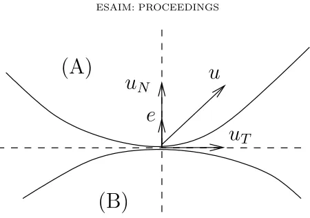
Figure 1. BodyAi _andBi _{with tangent and normal spaces}

velocity1

ui _{of A}i _{with respect to B}i _{and the force r}i _{applied by B}i _{onto A}i_{. The normal and tangential} components of a vectorxare denotedxN andxT respectively.

1.2.

Disjunction formulation

At each contact, we are given a coefficient of frictionµi _(0≤µi_{≤+∞), whose physical meaning is discussed} below in this subsection. Let us define the second-order cone with coefficientµi _{(the friction cone) as}

Kµi :={kx_Tk ≤µix_N} ⊂Rd, (1)

whose dual cone is (with the convention that 1

0 =∞and 1

∞ = 0)

K∗

µi =K1

µi ={kxTk ≤

1

µixN} ⊂R

d_{. (2)}

The productLof all friction cones and its dual coneL∗

are

L:= n

Y

i=1

Kµi⊂RndandL

∗

= n

Y

i=1

K_µ∗i ⊂Rnd. (3)

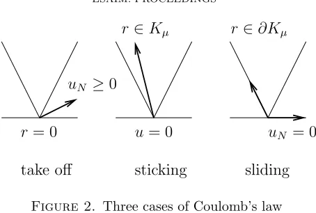
Then Coulomb’s law is usually formulated as adisjunction, that is, one of the three following cases must occur for eachi∈1, . . . n:

• take off : ri = 0 andui_N ≥0, • sticking : ri_∈K

µi andui= 0,

• sliding : ri _∈∂K

µi\0, ui_N = 0, ui_T 6= 0 opposed tori_T : ∃αi >0,ri_T =−αiui_T =−αui.

The physical meaning of Coulomb’s law is the following : the contact can cease (take off case), which means that the normal relative velocity is positive, but then there is no force between the two bodies : bodyBi_cannot push or pull onto bodyAi _{when the contact breaks. In other words, there is no attractive force, no glue between} the bodies (this models dry friction, without adherence) and no repulsive force either (a restitution coefficient will be added later to model rebound, but so far we are only discussing the contact force). The contact can also be maintained with zero relative velocity. In this case, the contact force can lie anywhere in its cone. Finally, if bodyAi_{is sliding on bodyB}i_{, the relative velocity is tangent. In this case, the friction force must be on the} boundary of its cone, and the tangent force must be collinear to the relative velocity with the opposite direction.

1_{As a general rule in this paper, bold letters will denote functions of time, whereas their discrete counterpart will be noted in}

r

= 0

u

= 0

u

= 0

r

∈

∂K

r

∈

K

u

≥

0

sticking

sliding

take off

Figure 2. Three cases of Coulomb’s law

e

e

u

K

r

r

˜

u

K

K

Figure 3. Change of variablesu→eu

This is often called the “maximimum dissipation principle” [15]. Note that the three cases are not mutually exclusive. For instance, the case whereri_{= 0 andu}i_{= 0 can be seen either as a (slow) take off or as sticking.} The value of parameterµi _{depends on the nature of the materials in contact (fromµ}i _{= 0 for a perfect contact} with no friction at all, toµi_{=∞for very rough and coarse surfaces).}

This formulation as a disjunction does not seem convenient neither theoretically nor practically. It suggests algorithms based on a tree search to explore all possibilities (3n_{if there arencontacts in the system) until one} is found which satisfies both Coulomb’s law and the equations of motions (derived below in section 2).

1.3.

Complementarity

Fortunately, this apparently disparate set of three different rules has a lot of structure, as described for instance by De Saxc´e-Feng [9]. Coulomb’s law does not derive from a potential, even non differentiable; this can be checked using the cyclic-monotonicity condition by Rockafellar [16] as in [9]. However, it does derive from a so-calledbipotential. The main trick is to change variables by setting

e

ui=ui+µi_kui

Tkei (4)

whereei_∈Rd _{is the unit normal vector fromB}i_toAi _{at contacti. Coulomb’s law can be expressed in a much} more compact way as a second-order cone complementarity constraint:

∀i∈1, . . . n,: Kµi ∋ri⊥eui∈K

∗

µi ⇐⇒ L∋r⊥eu∈L

∗

(5)

wherer:= (r1, . . .rn) andue := (ue1, . . .uen).

Indeed, (5) is equivalent to the following disjunction:

• either ri _{= 0, then automaticallyr}i_⊥uei _{for all eu}i _∈K∗

µi ; in turn, eui ∈K

∗

• oru_ei_{= 0 (so thatu}i _{= 0) and automaticallyr}i_⊥eui _{for allr}i_∈K

µi ; this is the “sticking” case

• orri _andeui _{are both non-zero, thenr}i_∈∂K

µi\0,eui∈∂K∗

µi\0 ; soµiuei_T =eui_N, andui_N = 0 withui_T

opposed tori_T ; this is the “sliding” case.

This simple idea of replacinguwith_euin the formulation yields an elegant and compact formulation of Coulomb’s law as a non-linear complementarity problem posed on two dual second-order cones. In the sequel, we will see that the complementarity formulation can be seen naturally as the optimality conditions (the Karush-Kuhn-Tucker system) of two mutually dual convex optimization problems coupled with a fixed-point equation.

1.4.

Impulse-velocity versus gap-force formulation

The relation between r and u described in subsection 1.2 is called the impulse-velocity formulation of Coulomb’s law, since complementarity occurs essentially between normal velocityuN and force (or impulse)r. It is adapted both to dynamic and quasi-static motion. On the other hand, the law is sometimes modelled using the so-called gap-force formulation, where complementarity occurs between the gap (defined as the distance, in some sense, between two potentially contacting objects) and the actual contact force between them. It is adapted to quasi-static motion, and has the advantage of enforcing non-penetrability explicitly, whereas the impulse-velocity formulation handles it implicitly through the fact that uN is maintained non-negative. As a consequence, the non-penetration constraints can be slightly violated in the course of the time integration, when the impulse-velocity formulation is used2_{. On the other hand, more convergence results are available for the}

impulse-velocity formulation [12, 18] and it is considered to lead to more stable time-integration schemes.

2.

Equations of motion

2.1.

Smooth Lagrangian mechanical systems

Let us consider a mechanical system in dimensiondwith finitely many degrees of freedom parametrized by

q(t)∈Rm. So far, only perfect (ie, without friction) bilateral constraints are allowed in the system (unilateral contact, possibly with friction, will be introduced later). Generalized velocities are defined as

v(t) := dq

dt(t)

and the equations of motion can be found using the formalism of Lagrangian Mechanics and the principle of virtual work ; they can be written in a general form as:

M(q(t))dv

dt(t) +N(q(t),v(t)) +Fint(t,q(t),v(t)) =Fext(t), (6)

where

• the matrix M(q), called the mass matrix, contains all the masses and the moments of inertia, in most applications one hasM(q)∈S++_n (ie,M(q) is a symmetric positive definite matrix),

• the vectorFint :R×Rn×Rn→Rnis the nonlinear force between bodies, called also the internal forces which are not necessarily derived from a potential,

• the vectorFext:R→Rn collects all the external applied loads, • and the vector

N(q,v) =



1

2

X

k,l

∂Mik

∂ql

+∂Mil

∂qk

−∂Mkl

∂qi

, i= 1. . . n



 (7)

collects the nonlinear inertial terms i.e., the gyroscopic accelerations.

2_{Non-penetrability can be retrieved a posteriori though, by projecting the solution onto the set of configurations with}

In the remaining part of the paper, the equation of motion (6) will be written in a more condensed form as

M(q(t))dv

dt(t) =F(t,q(t),v(t)), (8)

where the vectorF:R×Rn_×Rn _→Rn _{collects the termsFint,Fext andN(q,v).}

2.2.

Nonsmooth Lagrangian mechanical systems with unilateral contact and friction

Unilateral contraints can be introduced in the system and modelled using Lagrange multipliers, or using directly the contact forces written in the local frame at each contact. We will use the second option, which deals with variables that have a direct physical meaning. For each contacti∈1, . . . n, we label arbitrarily body

Ai _{and bodyB}i _{and we defineM}i

A=MBi as the contact point, withMAi attached to bodyAiandMBi attached to bodyBi_{. Then parametersq(t) can be used to find the position ofM}i

AandMBi :

∃fi

A, fBi : Rm−→Rd : MAi(t) =fAi(q(t)), MBi(t) =fBi(q(t)) and, differentiating with respect to time, their velocity

dMi A

dt = Jac[f

i

A](q(t))v(t),

dMi B

dt = Jac[f

i

B](q(t))v(t) (where Jac[·] denotes the Jacobian operator) and finally their relative velocityui_(t)

ui(t) =dM i A

dt − dMi

B

dt = (Jac[f

i

A]−Jac[fBi])(q(t))v(t).

Gathering all local relative velocities ui_{(t)(i = 1, . . . n) into u(t) = (u}1_{(t), . . . u}n_{(t)), this can be written in} matrix form as

u(t) =H(t)v(t), H(t) :=

  

Jac[f1

A]−Jac[f 1 B] Jac[f2

A]−Jac[f 2 B] ..

.

 

(q(t)) (9)

so that the vector of local velocities u(t) is a linear function of the generalized velocities v(t) (it could be affine, in case of a time-dependent parametrization or moving reference frame, without changing the rest of the argument).

Introducing the contact force3

ri_{(t) from B}i _{to A}i _{at each contacti, and gathering them in vector r(t) =} (r1_{(t), . . .r}n_{(t)), the principle of virtual work yields the new equation of motion as}4

M(q(t))dv

dt(t) =H(t)

⊤

r(t) +F(t,q(t),v(t)). (10) Equation (10), along with Coulomb’s law (4)-(5), form the continuous time problem. The model would be more complete with a restitution law (to allow for rebound) ; we will introduce it later in the discrete time model for convenience. Let us now turn to time discretization.

3_{Since the motion is nonsmooth, it should actually be an impulse and should be represented by a distribution, not a function,}

to allow for impacts. 4_{Once again, we write} dv

2.3.

Time discretization

In what follows, we assume that a time step δt is fixed and that we know an approximationqk, vk of the configuration q(tk),v(tk) at time tk (for some k, the number of timesteps already performed). We want to compute an approximation q, v of the configurationq(tk+1),v(tk+1) at time tk+1 := tk+δt. Assuming that H(q) andF(t,q,v) vary smoothly, we use a semi-implicit time discretization scheme with implicit discretization forr(t) and explicit discretization forH(q) andF(t,q,v). More precisely, we discretize (10) by

M(qk)(v(tk+1)−vk)≈H(tk)

⊤

r(tk+1)δt+F(tk, qk, vk)δt. (11) To simplify the notation, we set

M :=M(qk), f :=−M(qk)vk−F(tk, qk, vk)δt, H :=H(tk) and the discretized equation of motion writes

H⊤

r=M v+f (12)

where v ∈ Rm and r ∈ Rnd are the unknown generalized velocity (approximation for v(tk+1)) and contact

impulse (approximation for r(tk+1)δt) at time tk+1, and the rest is data depending only on values which are

known attk: M is anm×msymmetric positive definite matrix (again called the mass matrix),H is anm×nd matrix andf ∈Rmis a vector. Following Moreau [13], more elaborate time discretization schemes are possible which result in the same equation (12), so that the same method can be used to solve them.

To discretize Coulomb’s law (5), we also need a discrete version of the local velocities u(t); using the as-sumption that Hvaries smoothly, we replace H(tk+1) by H(tk) in (9) and we defineu, the approximation of u(tk+1), by

u:=H v. (13)

2.4.

Restitution law

In addition to friction, we allow for rebound between particles. Following Moreau [13] again, we adopt a simple rule based on a single coefficient ρi _{∈[0,1] so thatρ}i _{= 0 stands for a completely soft impact and no} rebound at all, whereasρi_{= 1 stands for a perfect rebound. Coefficientρ}i_{is introduced in the discretized model} by replacing, in the expression ofu_e, the normal local velocityui

N at contactibyuiN+ρiuiN,k(whereuiN,k is an approximation forui

N(tk)); in other words, we discretize (4) as follows

e

ui:=ui+ρiuiN,kei+µikuikei. (14)

The reason why this change in the expression ofu_edoes model rebound is the following. Wheneverri_{6= 0, there} holdsui

N+ρiuiN,k= 0 (sticking or friction case in Coulomb’s law), which means that

uiN =−ρuiN,k.

This is the simplest restitution law (sometimes called Newton’s law) , which states that the normal velocity after an impact is equal to minus the normal velocity before the impact amortized byρi_{. It is considered valid for} bodies with a geometry similar to spheres. On the contrary, for bodies with more complicated shape, it is known to be poor and can even entail creation of energy in the system [19], in contradiction with thermodynamics and common sense. For this reason, the chosen restitution law must be used with care and considered as a phenomenological rule more than a physical theory of impacts.

Let us introduce vectorc of (known) damped normal velocities attk by

c:= (ρ1_u1

vectorsof (unknown) sliding velocities attk+1by

s:= (ku1

Tk, . . . ,kunTk)∈Rn, (16)

and matrices

E:=

  

e1 _{0 . . .}

0 e2

..

. . ..

 

∈Rnd×n andD:=

  

µ1 _{0 . . .}

0 µ2

..

. . ..

 

∈Rn×n. (17)

Then, using (13), equation (14) can be written in matrix form as

e

u=Hv+E(c+Ds). (18)

Finally, we discretize Coulomb’s law formulated as a complementarity constraint (5) by

L∋r⊥eu∈L∗. (19)

2.5.

The one-step problem

Putting together the discretized equations of motion (12), the definition (18) of_eu, the discretized version of Coulomb’s law (19) and the definition (16) ofs, we get the following set of equations:

      

H⊤

r=M v+f [Newton’s law] (a)

e

u=Hv+E(c+Ds) [kinematics] (b)

L∋r⊥_eu∈L∗

[Coulomb’s law] (c)

si_=k

e

ui

Tk, i∈1, . . . n (d)

(20)

where we used in (d) the fact thatu_eT =uT. Our goal is to find a solution (v, u, r, s) to this set of equations for given dataH, M, f, E, c, D, L.

3.

Optimization-based formulation

In this section, we will view (20)-(a-c) as the optimality conditions of a minimization problem, where s is considered as a fixed parameter, in order to obtain the above-mentionned decomposition of the one-step problem into a parametric optimization problem coupled with a fixed-point problem.

3.1.

Optimality conditions of a conic problem

We first recall general sufficient optimality conditions for a convex optimization problem posed on a cone. Let K ∈ Rm _{be a closed convex cone,J : R}n _{−→R a differentiable convex function, andg : R}n _−→Rm _an affine function. If (¯v,¯r) solves the following system

∇J(v) = Jac[g](v)⊤

r

K∋g(v)⊥r∈K∗ (21)

then ¯v is an optimal solution to the following optimization problem

minJ(v)

3.2.

Application to the one-step problem

In (20), neglect equation (d) for the moment and considers as a fixed parameter. The key observation is that, setting

J(v) := 1 2v

⊤

M v+f⊤v and g(v) :=Hv+E(c+Ds)

we observe that the remaining equations (20)-(a-c) in (v,u, r˜ ) are the sufficient optimality conditions (22) for

the minimization problem

minJ(v) (quadratic, strictly convex)

g(v)∈L∗

(conic constraints). (23)

Unless this problem is infeasible, it has a unique solution v (M is positive definite). The correspondingu_e is then uniquely determined by (20)-(b) but observe thatris not unique if the rows ofH are linearly dependent. In fact, setting

J∗

(r) := 1 2r

⊤

(HM−1_H⊤

)r−(HM−1_{f −E(c+Ds))r}

in whichHM−1_H⊤

may not be invertible, standard duality theory says thatris given as a solution of the dual problem of (23), namely

minJ∗

(r) (quadratic, convex)

r∈L (conic constraints). (24)

Non-uniqueness ofris not surprising from a mechanical viewpoint, since a rigid body can be wedged and subject to non-unique contact forces ; the example of a bead in a corner below (subsection 5.3) shows such an example. As a consequence, the solution for velocities (v and u_e) are unique or non-existing, but the solution for forces (or impulses)rmust no be expected to be unique.

Using classical tricks [5], both problems can be reformulated into standard second order-cone programs (SOCP), that is to say optimization problems of the form

  

minc⊤

x (linear objective function)

Ax=b (affine constraints)

x∈Q_jKj (conic constraints)

whereKj are either second-order cones or polyhedral cones. The SOCP problem is well studied in the literature [2] and efficient algorithms and codes are available; we used the solver SeDuMi [20] for 3D problems (d= 3). For 2D problems (d= 2), the SOCP reduces to a quadratic program (QP) and any standard QP solver can be used. Finally, for each value ofs∈Rn+, we can either findv(s),ue(s), r(s) which satisfy (20)-(a-c) or prove that

no such triplet exist, for the computational price of solving a SOCP problem. The idea developed in section 4 is then to solve iteratively equation (20)-(d) :

si_=k

e

ui

T(s)k, i∈1, . . . n (25)

which is a fixed point equation. We could try to solve it using fixed-point iterations, but

• simple examples and experiments showed that the fixed point function is not a contraction in general, • it is actually possible to differentiate5 _{functions−→}

e

u(s) directionally, which allows use of Newton’s algorithm to solve the fixed point equation ; in the experiments done so far, the cost of computing the Jacobian matrix is cheap compared to the solution of (23) or (24), so there is no reason not to take advantage of the ability to differentiate the fixed point function.

For these reasons, we used a nonsmooth Newton’s algorithm to solve the fixed point equation (25). This algorithm is the object of the next section.

5_{This point needs a lot more theoretical explanations, which are beyond the scope of this paper. We only refer to subsection}

4.

Nonsmooth Newton algorithm

We now turn to the problem of solving the fixed-point equation (25). This can be done using a damped Newton’s algorithm : we first compute the Newton step, and then perform a line search in the Newton direction until the least-square function

φ(s) := 1 2

X

i

si− keuiT(s)k

2

decreases.

4.1.

Differentiation

In this subsection, we explain how we compute a generalized Jacobian matrix ofs−→ue(s) practically, and we keep as a future research direction to understand in what sense itis indeed a generalized Jacobian matrix. In other words, we postpone the analysis of the nonsmooth function s −→ ue(s). The idea, taken from the implicit functions theorem, is simply to derive the optimality conditions (20)-(a-c) with respect to s. Indeed, having solved (23), we obtain a list of those constraints in (1) and (2) which are active atv(s) andue(s); then we write

G(v(s),u_e(s), r(s), s) = 0⇔G(w(s), s) = 0 withw= (v,_eu, r)

where Gcollects (20)-(a-b), the active constraints at v(s) andue(s), and the orthogonality constrainteu·r= 0. We then differentiate with respect tos, and get

∂G ∂w

dw ds +

∂G ∂s = 0⇒

dw ds =−

_∂G

∂w

−1_∂G

∂s. (26)

To compute dw ds, hence

due

ds, it suffices to solve a set of linear systems (26).

4.2.

Initialization

Since we want to solve equation (25), we can restrict ourselves to s∈Rn+. However, for somes∈ Rn+, the

optimization problem (23) may be infeasible, so that functionφmay not be defined. If the friction coefficients

µi _{are all non-zero, however, it is always possible to find a feasible initial point for Newton’s algorithm, by} setting

s0:= max(−

ci

µi,0)

so thatv= 0 is feasible in (23). Ifµi_{= 0 for somei, it may not be possible to find an initial feasible point. For} instance, ifH is the null matrix,ci<0 andµi= 0 for somei, it is clear that no feasiblesexists.

4.3.

Computation of a Newton step

To find a fixed point ofF(s) := (kuei

T(s)k)i=1,...n, where F can be directionally differentiated according to subsection 4.1, we choose an initial s0 as in subsection 4.2, computeue(s) and a generalized Jacobian matrix

Jac[u_e](s), thenF(s) and a generalized Jacobian matrix Jac[F](s), and finally solve the linear equation

F(s) + Jac[F](s)ds=s+ds

to get the Newton step ds. Function eu(s) is evaluated again ats+ds, and if the least-square criterion φhas decreased, we replace s with by s+ds and loop. This is what happens almost all the time. Exceptionally however, the Newton step ds does not decrease the least-square criterionφ, or (23) is infeasible at s+ds so that φis undefined, ors+ds /∈Rn

h

θ

M

, m

θ

l

l

M

, m

e

e

O

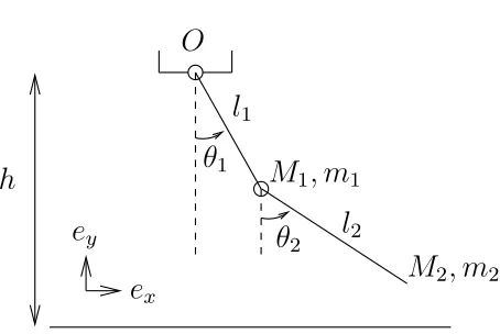
Figure 4. Double pendulum with friction

4.4.

Line-search

We use the Armijo rule for updating the stepds: the Newton stepdsis halved iteratively until φis found to decrease. This happens necessarily, since

∇φ(s)·ds= (F(s)−s)⊤(Jac[F](s)−I)(Jac[F](s)−I)−1(s−F(s)) =−kF(s)−sk2

so that the Newton direction ds is a descent direction for φ, unless F(s) = s which means that convergence already occured. Finally, the algorithm simply consists in minimizingφover its (not known explicitly) domain, using a damped nonsmooth Newton algorithm, until we hopefully reach a global optimum with value 0. Since

φdecreases at each iteration, the method is garanteed to be stable : it is not subject to cycling nor diverging brutally. However, it may stall and stop at a local minimum with non-zero value, even when a global optimum with value 0 exists. In this case, the method fails; such a counterexample is given in subsection 5.4.

5.

Numerical examples

In this section, we give a few simple examples and counterexamples. The one-step problem (20) is written explicitly for the double pendulum with friction in two dimensions, to illustrate the approach. The algorithm is also run on random instances of problems, to see how it performs in various situations. Finally, counterexamples are given which show that the solution to (20) is not unique in general (example of a bead wedged in a corner) and that the algorithm is not garanteed to converge to an actual solution (global minimum of 0 for functionφ) when one exists, since the damped Newton algorithm may stop at a local minimum ofφ.

5.1.

Double pendulum with friction

In this subsection, we illustrate the method by writing and solving numerically the problem for a double pendulum with friction, as depicted on figure 4. The pendulum is made of two punctual massesm1 andm2in

M1 andM2. M1 is linked to the ceiling by a rigid rod of lengthl1 with no mass and a perfect ball joint. M2

is linked to M1by a rigid rod of length l2 with no mass and a perfect ball joint. The only external load is the

weight due to gravityg∈R2. The system has two degrees of freedom, we parametrize it by q= (θ1, θ2). The

kinetic energy is

T := 1 2m1M˙1

2

+1 2m2M˙2

2

=1

2(m1+m2)l

2 1θ˙1

2

+1

2m2(2l1l2cos(θ1−θ2) ˙θ1θ˙2+l

2 2θ˙2

2

−3 −2 −1 0 1 2 3 −3

−2.5 −2 −1.5 −1 −0.5 0

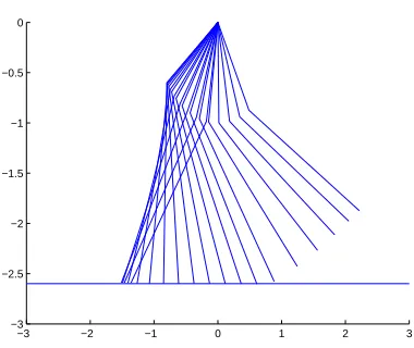
Figure 5. A trajectory for the double pendulum with friction

IfM2·ey≤ −h,M2 is in contact with the ground, and

H= dM2

dq =

l1cosθ1 l2cosθ2

l1sinθ1 l2sinθ2

(otherwise, if M2 does not touch the ground, H is the empty matrix) and the Lagrange equations of motions

write

d dt

_∂T

∂q˙

−∂T

∂q =m1 dM1

dq

⊤

g+m2

dM2

dq

⊤

g+H⊤

r

which, after some computations, is exactly in the form (10) with

M=

(m1+m2)l12 m2l1l2 cos(θ1−θ2)

m2l1l2 cos(θ1−θ2) m2l22

, N=m2l1l2sin(θ1−θ2)

˙

θ2 2

−θ˙1 2

!

,

Fext=

l1(m1+m2) (cos(θ1)gx+ sin(θ1)gy)

l2m2(cos(θ2)gx+ sin(θ2)gy)

andFint= 0.

For m1 = m2 = 1 (in kilograms), l1 = 1, l2 = 2, h = 2.6 (in meters) µ = 0.01 (dimensionless) andρ = 0

(dimensionless, no restitution), we obtain the trajectory drawn on figure 5. The pendulum swings from right to left (and then back) and its position is depicted every 0.2 seconds.

5.2.

Random instances

In order to test the algorithm for various data, we performed experiments with random instances of the one-step problem. We used different values forn (number of contacts) andm(number of degrees of freedom), uniformly distributed values for the coefficientsµi _{(i= 1, . . . m) in the interval [µ}

min, µmax], mass matricesM randomly generated by matlab’s functionsprandsym, and matricesH randomly generated by matlab’s function

a few iterations, with satisfying precision. These results are encouraging, but one must keep in mind that each iteration is costly (one SOCP to solve) and that these random problems may not be typical of the situations met in real-world instances.

Table 1. Random instances in 2D

instance n m µmin µmax #iter φ(sinitial) φ(sf inal)

1 10 40 0.5 2 1 42.3 3.1e-30

2 20 80 0.5 2 2 38.8 8.4e-27

3 30 120 0.5 2 3 166.1 1.6e-28

4 40 160 0.2 3 3 184.6 1.2e-27

5 50 200 0.2 3 1 303.9 2.6e-27

6 60 240 0.2 3 4 610.8 7.8e-29

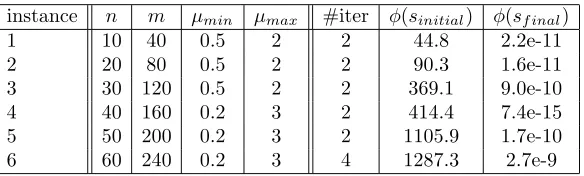
Table 2. Random instances in 3D

instance n m µmin µmax #iter φ(sinitial) φ(sf inal)

1 10 40 0.5 2 2 44.8 2.2e-11

2 20 80 0.5 2 2 90.3 1.6e-11

3 30 120 0.5 2 2 369.1 9.0e-10

4 40 160 0.2 3 2 414.4 7.4e-15

5 50 200 0.2 3 2 1105.9 1.7e-10

6 60 240 0.2 3 4 1287.3 2.7e-9

5.3.

Bead in a corner

The example of a bead wedged in a corner shows that the one-step problem (20) may have several isolated solutions. Consider the situation of figure 6 : a bead is in contact with two walls, with friction at contact points, and an external force is used to pull the bead away from the corner. The bead is initially at rest (no movement) and we want to compute the first timestep, that is to say, to solve the first one-step problem. From a mechanical viewpoint, it is quite clear that two outcomes are possible :

• either there are contact forces, which counterbalance the applied external load ; the bead does not move, it is wedged by friction forces

• or there are no contact forces, the bead is pulled away and has nonzero velocitiesu1and u2.

Both situations are physically acceptable, and indeed there are two isolated minima with value 0 in functionφ

~

f

K

K

u

u

~

f

r

r

_K

K

Figure 6. A bead wedged in a corner

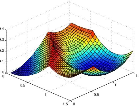
Figure 7. Piecewise quadratic functionφfor the bead in a corner

5.4.

Bad boy for Newton’s algorithm

In this subsection, we give a counter-example which shows that even for the simplest case of one contact in two dimensions, the algorithm may converge to a point which is not a solution to the one-step problem (20). Consider the following data (for a mechanical system with two degrees of freedom):

M =

2 −3

−3 5

, f =

−1 0

, H =

1 0 0 1

, µ= 1, c= 0

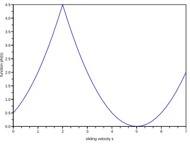
then φ : R+ −→ R+ is the function depicted on figure 8. There is a local minimum fors = 0 with nonzero value, and a global minimum with zero value ats= 5. The function restricted to [0,2] or [2,∞[ is convex (and quadratic, sinced= 2). If our minimization algorithm forφis initialized withs0<2, it will converge to s= 0

and fail. If it is initialized withs >2, it will converge tos= 5 and succeed. If one chooses exactlys0= 2, the

0 1 2 3 4 5 6 7 0.0

0.5 1.0 1.5 2.0 2.5 3.0 3.5 4.0 4.5

sliding velocity s

function phi(s)

Figure 8. Piecewise quadratic functionφwith a local minimum in 0 which is not a solution

Conclusion

Using a classical impulse-velocity formulation of Coulomb’s law to model friction, a phenomenological rule to model restitution, and a semi-implicit time discretization scheme, we write the discretized equations of motion for a Lagrangian mechanical system subject to unilateral contact with friction. This results in a system of equations mixing linear, non linear and complementarity equations (the one-step problem), with interesting structure : it can be equivalently formulated as a parametric convex minimization problem coupled with a fixed point equation. This equivalent reformulation opens the way to a specific algorithm to compute a solution for the one-step problem. Numerical experiments illustrate the method and show the feasibility of the proposed algorithm. We keep as a research direction to better understand the properties of the nonsmooth function φ

used for minimization, and the theoretical properties of the algorithm. In particular, it seems that althoughφis nonsmooth, Newton’s algorithm achieves superlinear convergence (as observed in the experiments). Future work will also include comparisons with existing techniques, based either on projected Gauss-Seidel like algorithm or on Newton’s algorithm.

The author wishes to thank Vincent Acary, Claude Lemar´echal and J´erˆome Malick for their help and support and the organizers of Canum 2008 for inviting him to publish this paper.

References

[1] P. Alart and A. Curnier. A mixed formulation for frictional contact problems prone to Newton like solution methods.Comput. Methods Appl. Mech. Eng., 92(3):353–375, 1991.

[2] F. Alizadeh and D. Goldfarb. Second-order cone programming.Math. Prog. Ser. B, 95:3–51, 2003.

[3] M. Anitescu and F.A. Potra. Formulating dynamic multi-rigid-body contact problems with friction as solvable linear comple-mentarity problems.Nonlinear Dyn., 14(3):231–247, 1997.

[4] Brian Armstrong-H´elouvry.Control of machines with friction.The Kluwer International Series in Engineering and Computer Science. 128. Dordrecht: Kluwer Academic Publishers Group. VIII, 173 p. , 1991.

[5] Aharon Ben-Tal and Arkadi Nemirovski. Lectures on modern convex optimization. Analysis, algorithms, and engineering applications.MPS/ SIAM Series on Optimization. Philadelphia, PA: SIAM, Society for Industrial and Applied Mathematics. Philadelphia, PA: MPS, Mathematical Programming Society, xvi, 488 p. , 2001.

[6] Bernard Brogliato.Nonsmooth mechanics. Models, dynamics and control. 2nd ed.Communications and Control Engineering Series. London: Springer. xx, 552 p., 1999.

[7] Bernard Brogliato and Vincent Acary.Numerical methods for nonsmooth dynamical systems. Springer, 2008.

[9] G. De Saxc´e and Z. Q. Feng. The bipotential method: a constructive approach to design the complete contact law with friction and improved numerical algorithms.Math. Comput. Modelling, 28(4-8):225–245, 1998.

[10] Franck Jourdan, Pierre Alart, and Michel Jean. A Gauss-Seidel like algorithm to solve frictional contact problems.Comput. Methods Appl. Mech. Eng., 155(1-2):31–47, 1998.

[11] Danny M. Kaufman, Timothy Edmunds, and Dinesh K. Pai. Fast frictional dynamics for rigid bodies.ACM Trans. Graph., 24(3):946–956, 2005.

[12] Manuel D.P. Monteiro Marques.Differential inclusions in nonsmooth mechanical problems. Shocks and dry friction.Progress in Nonlinear Differential Equations and their Applications. 9. Basel: Birkh¨auser. x, 179 p. DM 98.00; S 764.40; sfr. 88.00 , 1993.

[13] J-J. Moreau. Mod´elisation et simulation de mat´eriaux granulaires. InActes du 35`eme Canum, 2003.

[14] J-J. Moreau. Mod´elisation et simulation de mat´eriaux granulaires. InActes du 6`eme Coll. Nat. Calc. Struct., 2003.

[15] J.J. Moreau. Unilateral contact and dry friction in finite freedom dynamics. Nonsmooth mechanics and applications, CISM Courses Lect. 302, 1-82 (1988)., 1988.

[16] R.T. Rockafellar.Convex analysis.Princeton, N. J.: Princeton University Press, XVIII, 451 p. , 1970.

[17] J.C. Simo and T.A. Laursen. An augmented Lagrangian treatment of contact problems involving friction.Comput. Struct., 42(1):97–116, 1992.

[18] David E. Stewart. Rigid-body dynamics with friction and impact.SIAM Rev., 42(1):3–39, 2000.

[19] W.J. Stronge. Unraveling paradoxical theories for rigid body collisions.J. Appl. Mech., 58(4):1049–1055, 1991. [20] Jos F. Sturm. Using SeDuMi 1. 02, a MATLAB toolbox for optimization over symmetric cones.Opt. Meth. Soft., 1999. [21] Otis R. Walton. Numerical simulation of inelastic frictional particle-particle interactions.Roco, M.C. (Ed.), Particulate