Multiscale modelling of endocrine systems: new insight on the gonadotrope axis

C. Besse, O. Goubet, T. Goudon & S. Nicaise, Editors

MULTISCALE MODELLING OF ENDOCRINE SYSTEMS: NEW INSIGHT ON

THE GONADOTROPE AXIS

Fr´

ed´

erique Cl´

ement

Abstract. In vertebrates, the gonadotrope axis is made up of the hypothalamus, belonging to the central nervous system, the pituitary gland and the gonads. These organs communicate with one another within entangled endocrine loops. From a dynamical viewpoint, the gonadotrope axis exhibits remarkable features, such as the pulsatile mode of secretion of the master reproductive hormone GnRH (gonadotropin releasing hormone) and the permanent renewal of the gonadic tissues related to the maturation of the germ cell lines. We will present a multilevel and multiscale modelling approach of the gonadotrope axis focusing on the ovulation process. On the gonadic level, we address the question of the selection of ovarian follicles within the framework of controlled conservation laws. We have to deal with a 2D EDP with integro-differential expressions in the velocity and source terms. On the hypothalamic level, we design a model of GnRH secretion within the framework of weakly coupled nonlinear oscillators. The model outputs reproduce the transition from the pulsatile to the surge pattern and the changes in pulse frequency. To explain the behaviour of the model and meet qualitative and quantitative endocrinological specifications, we explore the whole sequence of bifurcations occurring within the model.

R´esum´e. Chez les vert´ebr´es, l’axe gonadotrope est constitu´e par l’hypothalamus (structure du sys-t`eme nerveux central), l’hypophyse et les gonades, dont les activit´es sont coordonn´ees par des boucles de r´etrocontrˆole endocrines. Le fonctionnement de ce syst`eme exhibe des propri´et´es remarquables sur le plan dynamique, telles que le caract`ere pulsatile de la s´ecr´etion de la GnRH (gonadotropin releasing hormone) par les neurones hypothalamiques, et le remaniement permanent (au cours de la vie reproductive) des tissus gonadiques, en liaison avec la maturation des cellules germinales.

Il s’agit ici de pr´esenter une approche de mod´elisation et de contrˆole multi-´echelles et multi-niveaux de l’axe gonadotrope. Au niveau gonadique, nous d´ecrirons un mod`ele multi-´echelles du processus de s´election des follicules ovulatoires, au sein de la population de follicules ovariens en croissance, rentrant dans le cadre des lois de conservation contrˆol´ees. Au niveau hypothalamique, nous pr´esenterons un mod`ele de s´ecr´etion de la GnRH, dans le cadre du couplage d’oscillateurs non lin´eaires. Les sorties du mod`ele reproduisent non seulement la transition entre r´egime pulsatile et d´echarge ovulatoire, mais aussi l’acc´eleration en fr´equence avant la d´echarge, et l’existence d’une pause apr`es la d´echarge. Nous ´etudions la s´equence compl`ete de bifurcations sous-jacentes au mod`ele, afin de respecter fid`element les sp´ecifications qualitatives et quantitatives du cahier des charges endocrine, qui portent sur les rapports en dur´ee, amplitude et fr´equence, entre les diff´erents ´ev´enements s´ecr´etoires.

∗_{This work falls within the large scale project REGATE (REgulation of the GonAdoTropE axis)} 1 _{INRIA Paris-Rocquencourt Research Centre}

Domaine de Voluceau, Rocquencourt BP 105, 78153 Le Chesnay Cedex, France

c

EDP Sciences, SMAI 2009

Introduction

Physiological background.In vertebrates, the neuroendocrine axes play a major part in controlling the main physiological functions (metabolism, growth, development and reproduction) and integrating internal or ex-ternal environmental factors. The connection between the central nervous system and the endocrine system takes place on the level of the hypothalamus, where specific neurons are able to secrete hormones that target the pituitary gland. In birds and mammals, a dedicated portal system (the pituitary portal system) joins the hypothalamus and pituitary gland together. The anterior lobe of the pituitary gland (adenohypophysis) pro-duces different hormones, which target either other endocrine glands (releasing their hormones directly into the bloodstream), exocrine glands (releasing their hormones into dedicated ducts) or non-secreting organs. Each neuroendocrine axis is named according to its most downstream component: thyroid gland (thyreotrope axis), adrenal glands (corticotrope axis), gonads - ovaries in females, testes in males -(gonadotrope axis), mammary gland (lactotrope axis), muscles, bones and cartilages (somatotrope axis).

In the sequel, we will focus on the gonadotrope axis (see Figure 1). The reproductive function is a complex, tightly controlled physiological function, subject to many environmental cues such as the daylength, food avail-ability and social interactions, as well as to internal signals such as stress or metabolic status. If the conditions are favourable, specific hypothalamic neurons secrete, in a pulsatile manner, the GnRH (gonadotrophin releas-ing hormone), the ”conductor” of the gonadotrope axis. The pulsatile GnRH secretion pattern ensues from the synchronisation of the secretory activity of individual GnRH neurons. The release of GnRH into the pituitarian portal blood induces the secretion of the luteinising hormone (LH) and follicle-stimulating hormone (FSH) by the gonadotroph cells within the pituitary gland. The gonadotrophins LH and FSH control the development of germinal cells within the gonads and their secretory activity. In turn, hormones secreted by the gonads (steroid hormones such as androgens, progestagens and oestrogens or peptidic hormones such as inhibin) modulate the secretion of GnRH, LH and FSH within entangled feedback loops. In females, the GnRH secretion pattern dramatically alters once per ovarian cycle, resulting in the GnRH surge characterised by massive continuous release of GnRH. The GnRH surge is responsible for the LH surge that triggers ovulation, leading to the release of fertilisable oocytes from ovarian follicles selected for ovulation.

Figure 1. Reproductive system. The gonadotrope axis involves the hypothalamus (within the central nervous system), the pituitary gland and the gonads: ovaries in females, testes in males. These organs communicate with one another within entangled endocrine feedback loops, involving the GnRH (gonadotrophin releasing hormone), the gonadotrophins, FSH (follicle stimulating hormone) and LH (luteinising hormone), and gonadic steroid and peptidic hormones, such as progesterone, oestradiol, testosterone and inhibin (Courtesy of D. Monniaux).

regard to a specific context of biological knowledge and data. We will first present an instance of multiscale modelling of coupled structured populations and its application to the selection process of ovarian follicles for ovulation. This model focuses on the ovarian level of the gonadotrope axis, even if it takes into account the ovarian feedback onto both the hypothalamus and pituitary gland. Its main output consists in predicting the ovulation rate (number of ovulating follicles). We will then introduce an instance of weakly coupled relaxation oscillators and its application to the secretion dynamics of hypothalamic GnRH. This model focuses on the hypothalamic level; its main output consists in predicting ovulation chronology (time of ovulation onset).

1.

Multiscale modelling of coupled and structured cell populations : the

selection process of ovarian follicles towards ovulation

1.1.

Model formulation

1.1.1. Physiological basis and working hypotheses

The ovulation process is the endpoint of follicular development, the process of growth and functional mat-uration undergone by ovarian follicles, from the time they leave the pool of primordial follicles until ovulatory stage. Its biological meaning is to release one (in mono-ovulating species) or several (in poly-ovulating species) fertilisable oocyte(s) enabled to subsequent embryo development. Actually, very few follicles reach an ovula-tory size; most of them undergo a degeneration process, known as atresia. The species-specific ovulation rate (number of ovulatory follicles) results from an FSH-dependent follicle selection process.

the pituitary gland is in turn modulated by granulosa cell products such as oestradiol and inhibin. This feedback is responsible for reducing FSH release, leading to the degeneration of all but those follicles selected for ovulation. Formally, the selection process falls within the field of population dynamics as a process of competition for FSH resource, whose level is determined by some trait of the population itself.

Accordingly, we have proposed a mathematical model, using both multi-scale modelling and control theory concepts, to describe the follicle selection process [10]. For each follicle, the cell population dynamics is ruled by a conservation law with variable coefficients, which describes the changes in age and maturity of the granulosa cell density. A control term, representing FSH signal, intervenes both in the velocity and loss terms of the conservation law. Two acting controls are distinguished: a global control resulting from the ovarian feedback and corresponding to FSH plasmatic levels, and a local control, specific to each follicle, accounting for the modulation in FSH bioavailability due to follicular vascularisation. Besides, cells are characterised by their position within or outside the cell cycle and their sensitivity to FSH. This leads to distinguish 3 cellular phases within the granulosa cell population. Phases 1 and 2 correspond to the proliferation phases (describing respectively the G1 phase and S to M phases of the cell cycle), and phase 3 corresponds to the differentiation phase, after cells have exited the cell cycle (see Figure 2).

G1

M _G2

S

D

AGE

sensitive to FSH

Apoptosis

insensitive to FSH sensitive to FSH

x2

SM D

G1

Flow chart Cell cycle

MATURITY

Figure 2. Structure of the cell population in ovarian follicles. The cell cycle consists of the G1 and SM phases. Cells in phase D have exited the cell cycle. Entry into apoptosis arises from either the G1 or D phase, where the cells are sensitive to the control exerted by FSH.

1.1.2. Detailed model formulation

To describe the changes in the cell density within an ovarian follicle, we consider a functional space (rather than the physical space), where the position of a cell at time t∈[0, T] (T >0) is defined by its age and maturity. The cell ageais a marker of progression within the cell cycle (in phases 1 and 2) and evolves as timetoutside the cycle (in phase 3). The duration of phase 1 is a1 >0 and the total cycle duration isa2 (so that phase 2

duration is a2−a1 >0). The maturity markerγ is used to discriminate between the cycling and non-cycling

cells by comparison to a thresholdγsand to characterise the cell vulnerability towards apoptosis. Phases 1, 2,

and 3 correspond respectively to ranges in the values of (a, γ) in the following open sets of the age-maturity plane:

Ω1,k=]ka2, ka2+a1[×]0, γs[, Ω2,k=]ka2+a1,(k+ 1)a2[×]0, γs[, Ω3,k=]k,(k+ 1)a2[×]γs, γmax[

The cell population in a follicle,f, is represented by cell density functions,φk

f,j(a, γ, t), defined on each cellular

phaseQj,k,j = 1,2,3,k= 0,1, . . .as solutions of the following conservation laws:

∂φk f,j

∂t +

∂gf(uf)φkf,j

∂a +

∂hf(γ, uf)φkf,j

∂γ =−λ(γ, U)φ

k

f,j inQj,k, j= 1,2,3, k= 0,1, . . . (1)

In phases 1 and 3, both a global control,U, and a local control,uf, act on the velocities of aging (gf function,

locally controlled in phase 1) and maturation (hf function, locally controlled in phases 1 and 3) as well as on

the loss term (λapoptosis rate, globally controlled in phases 1 and 3). Phase 2 is uncontrolled and corresponds to completion of mitosis after a pure delay in age,a2−a1 (no cell can leave the cycle here). The velocity and

source terms are given by the following expressions (all parameters are real positive numbers):

gf(uf) = τgf(1−g1(1−uf)) in Ω1,k

hf(γ, uf) = τhf(−γ2+ (c1γ+c2)(1−exp(−uf/u¯))) in Ωj,k, j= 1,3

λ(γ, U) = ωλ(γ)(1−U) in Ωj,k, j= 1,3 (2) gf(uf) = τgf in Ωj,k, j= 2,3 hf(γ, uf) =λ(γ, U) = 0 in Ω2,k

In complement to the local control exerted by uf on the cell cycle exit, a global control is exerted by U

(U ≤1) on the cell vulnerability towards apoptosis, in a zone surroundingγs, through the function

ωλ(γ) =Kexp

−γ−γs

¯ γ

2

in (2).

The formulation of the model is completed by the boundary conditions forφk

f,1,φkf,2 andφkf,3,t∈]0, T[:

gf(γ, uf)φkf,1(ka2, γ, t) =

2τgfφk_f,−21(ka2, γ, t), fork≥1,

0, fork= 0 forγ∈]0, γs[

φk

f,1(a,0, t) = 0, fora∈]ka2, ka2+a1[

τgfφkf,2(ka2+a1, γ, t) = gf(γ, uf)φkf,1(ka2+a1, γ, t), forγ∈]0, γs[

φkf,2(a,0, t) = 0, fora∈]ka2+a1,(k+ 1)a2[

φk

f,3(ka2, γ, t) =

φk_f,−₃1(ka2, γ, t), fork≥1,

0, fork= 0 , forγ∈]γs, γmax[

φkf,3(a, γs, t) =

φk

f,1(a, γs, t), fora∈[ka2, ka2+a1[

0, fora∈[ka2+a1,(k+ 1)a2[

Finally, initial conditions are stated as:

φkf,j(a, γ,0) =φkf0(a, γ)|Ωj,k, j= 1,2,3.

The feedback exerted by the ovaries on FSH secretion defines a closed-loop system. The global controlU can be interpreted as FSH plasmatic level. The local control uf represents intra-follicular bioavailable FSH levels

and is given as a proportion of U. Define theγ moment operatorMp _as:

Mp_{(ϕ)(t) =} Z γmax

0

Z amax

0

γp_{ϕ(a, γ, t)dadγ p∈ {0,1}}

For sake of legibility, we also introduce the notationφf as:

The zero-order momentM0_(φ

f) corresponds to the whole follicular cell number. The global maturitiesM1(φf)

on the follicular scale, andM1(X

f

φf) on the ovarian scale, will be used to define the two-scale feedback control:

U = S(M1(X

f

φf)) +U0

uf = bf(M1(φf)).U

whereS(µ) = Us+

1−Us

1 + exp (c(µ−m)),

bf(µ) = min

b1+exp

b2µ

b3 ,1

.

The decreasing sigmoid function S accounts for the ovarian negative feedback on FSH; U0(t) is a potential

exogenous entry1. Function bf makes uf increase with the maturity of follicle f, up to its reaching FSH

plasmatic values. U andbf are normalised (0< b1, Us<1), so that 0≤uf ≤U ≤1 +U0.

The shape of the whole domain is illustrated, together with a sketch of the velocity field, in Figure 3.

Ω

Ω

Ω

Ω

Ω

. . .

Ω

Ω

a₁ a₂

γ γ_max

s

Figure 3. Sketch of the velocity field on the domain. The sign of the local vertical velocities depends on the current value of the local control uf. The sign of the local horizontal velocities is always positive. The dotted lines delimits the zone where cells are intrinsically vulnerable to apoptosis.

The well-posedness of the whole model is discussed in [9], in the case where the control values are in steady-state (which just amounts to define them as function of time on successive small time intervals) and regularised expressions for the velocities. The reasoning is based on considering a sequence of subproblems defined on each Ωi,k{k=0,...,N−1}, and tracking the traces of the solutions on the outward boundaries of the Ωi,k domains.

1.2.

Numerical scheme and simulations

1.2.1. Numerical scheme

We briefly describe the numerical scheme, based on high-resolution, wave-propagation algorithms developed by RJ LeVeque for multi-dimensional hyperbolic systems [16]. We first expand the derivative terms in equation

1_{It can be shown that, as soon asU}

(1) in order to obtain the color equation:

∂φf(a, γ, t)

∂t +gf(uf)

∂φf(a, γ, t)

∂a +hf(γ, uf)

∂φf(a, γ, t)

∂γ =−λ(γ, U)φf(a, γ, t)−

∂hf(γ, uf)

∂γ φf(a, γ, t), (3)

and consider a two-dimensional cartesian mesh made of cells

Cij =

a_i−1 2, ai+

1 2

×γ_i−1 2, γi+

1 2

with lengths ∆ai=ai+1 2 −ai−

1

2, ∆γi=γj+ 1 2 −γj−

1 2.

Let Φn

ij be an approximation of the solution in the sense of finite volumes:

Φnij =

1 ∆ai

1 ∆γi

Z γ_j+ 1 2

γ_j

−12

Z a_i+ 1 2

a_i

−12

φf_i(a, γ, tn)dadγ

The Riemann problems normal to each cell edge at the cell interfacesai−1

2 andγi− 1 2 read:

Φn_i−1 2,j=

(

Φn

i−1,j ifa < ai−1 2,

Φn

i,j ifa > ai−1 2,

Φn_i,j−1 2 =

(

Φn

i,j−1 ifγ < γj−1 2,

Φn

i,j ifγ > γj−1 2,

We now use a fractional-step method to solve equation (3). Hence, we will first solve the homogeneous equation to obtain the solution Φ∗

ij that we will then use to update the solution of the whole equation at time tn+1

according to:

∂Φn+1 ij (a, γ, t)

∂t =−λ(γ, U)Φ

∗

ij(a, γ, t)−

∂hf(γ, uf)

∂γ Φ

∗

ij(a, γ, t)

Assuming that we know the speeds on the cell edges, the homogeneous equation becomes an advection equation with constant terms on each interface, for which the solution of the Riemann problem is well-known. For instance, at (ai−1

2, γj) we have:

∂Φ∗

ij(ai−1 2, γj, t)

∂t +gi−12,j(uf) ∂Φ∗

ij(ai−1 2, γj, t)

∂a +hi−12,j(uf) ∂Φ∗

ij(ai−1 2, γj, t)

∂γ = 0

where g_i−1

2,j = gf(ai− 1

2, γj, uf) and hi− 1

2,j = hf(ai− 1

2, γj, uf). The numerical solution of the homogeneous

equation can thus be updated at time tn+1=tn+ ∆t according to edge-centered numerical flux fonctions:

Φ∗_ijn+1= Φnij−

∆t

∆ai

A+∆Φi−1 2,j+A

−_∆Φ

i+1 2,j

− ∆t ∆γj

B+∆Φi,j−1 2 +B

−_∆Φ

i,j+1 2

− ∆t ∆ai

˜

F_i+1 2,j−

˜

F_i−1 2,j

− ∆t ∆γj

˜

G_i,j+1 2 −

˜

G_i,j−1 2

where ∆Φi−1 2,j≡Φ

n

ij−Φni−1,j. The horizontal flux difference is split into a left-going fluctuationA−∆Φi+1 2,j

and a right-going fluctuationA+_∆Φ i+1

B+_∆Φ i,j−1

2 and a down-going fluctuationB −_∆Φ

i,j+1

2, according to the following expressions:

A±∆Φ_i−1

2,j = g ±

i−1 2,j

(Φi,j−Φi−1,j)

B±∆Φi,j−1

2 = h

±

i,j−1 2

(Φi,j−Φi,j−1)

The fluctuations are computed from the wave structure determined by solving the Riemann problems on the interfaces normal to the cells. The left (resp. right)-going fluctuations capture the net effect of all left (resp. right) waves entering the cell from the left (resp. right).

Besides these first-order terms, the ˜F and ˜Gfluxes are used to perform second order corrections including cross-derivatives terms. They take into account the contributions of up-going and down-going transverse fluc-tuations, as well as second order corrections of the one-dimensional fluxes using adequate flux limiters. They are computed according to the following algorithm:

˜

G_i,j−1

2 := 0

˜

G_i,j−1 2 :=

˜

G_i,j−1 2 +

1 2

hi,j−12

I− ∆t

∆γ

hi,j−12

(Φij−Φi,j−1)

˜

Gi,j+1 2 :=

˜

Gi,j+1 2−

∆t

2∆ah + i,j+1

2g + i−1

2,j∆Φi− 1 2,j

˜

G_i,j−1 2 :=

˜

G_i,j−1 2 −

∆t

2∆ah

−

i,j−1 2

g_i+₋1 2,j

∆Φ_i−1 2,j

˜

Gi−1,j+1 2 :=

˜

Gi−1,j+1 2 −

∆t

2∆ah + i−1,j+1

2 g_i−₋1

2,j

∆Φi−1 2,j

˜

G_i−1,j−1 2 :=

˜

G_i−1,j−1 2 −

∆t

2∆ah

−

i−1,j−1 2

g−_i−1 2,j

∆Φ_i−1 2,j

We have considered the non conservative form of equation (1), which amounts to a 2D advection equation with variable coefficients, gf andhf, and ”augmented” source term −φf

∂

∂γhf+λ(γ, U)

. This approach is described in details in [8] and derives directly from the algorithm presented in [16]. The source term is handled by a fractional step (Godunov splitting) method. An alternative choice would consist in using the source term to modify the flux difference before performing the wave decomposition, as described in [1]. However care will have to be taken before applying this method to our case since it is not really suited for flux functions that may change signs.

1.2.2. Numerical simulations

This scheme has been implemented within the academic software environment bearclaw2, where it is coupled to a dedicated adaptative mesh refinement (AMR) algorithm [3]. Since the computing time is quite limiting, we are currently adaptating a MPI-version of the code. Figure 4 illustrates simulation snapshots on the inverse L-shaped domain merging the 3 cellular phases. The succession of the kth cell cycles is accounted for by periodic inward boundary conditions on the left edge of phase 1. Hence, instead of being unrolled in a modulo

a2 description as illustrated in Figure 3, the bottom part of the domain is somehow rolled upon itself and the

age is reset at each new cell cycle. The CFL value turns around 0.6, so that ∆t≈min (0.6 ∆ai/gij,0.6 ∆γi/hij).

Due to the AMR, its value is indeed not strictly constant. The panels of Figure 4 correspond to different stages in the development of an ovulatory follicle, that span several days from the initially proliferative stage to the terminally differentiated one. The reference time is given by the duration of the cell cycle (a2, which roughly

amounts to 12 hours) in the case where the transit time within the G1 phase is not controlled (da_dt = 1).

1.3.

Control of ovulation rate

1.3.1. From models to experiments and vice-versa

Running simulations allows to predict the outcome of follicular development (ovulation and ovulation rate, or anovulation) for a given parameter combination. It can also be useful in testing control strategies. For instance, preliminary trials of exogenous FSH administration to compensate the drop in FSH suggest that it is possible to tune the ovulation rate finely [10].

Even if the computing time has prevented us from studying large size follicle cohorts up to now, the model can help interpret biological knowledge and suggest experiments, since it accounts for the intricate relation-ships between follicle growth and differentiation with FSH secretion from the pituitary gland and triggering of ovulation by the GnRH surge from the hypothalamus.

The more directly observable variable corresponds to the cell number in each phase (zero-order moment of the density φif,i=1...3). It can be compared to data providing information on the whole follicle cell

num-ber - M0_(φ

f)(t) -, or the growth fraction - proportion of proliferating cells within the whole cell population:

M0_(φ

1f)(t) +M0(φ2f)(t)/M0(φf)(t) -. In a previous model-driven experiment [7, 21], we have shown that

the growth fraction decreases throughout follicular development and also that the drop in the growth fraction differs in mono-ovulating situations from poly-ovulating ones. The underlying notion of differential manage-ment of proliferating resources can be further explained from the current model framework as differences in the ratio of aging and maturation velocity time constants. The multi-level property of the model allows to propose an integrative scenario for the control of ovulation rate, where multiple ovulations ensue from the combined increased follicular sensitivity to FSH, leading to lower whole follicle cell numbers at ovulation time [12], de-creased sensitivity of the pituitary gland to ovarian negative feedback [15] and/or dede-creased sensitivity of the hypothalamus to ovarian positive feedback [2]. Whatever the ovulation rate, the ”losing” atretic follicles are those whose cells are confined within the maturity zone of vulnerability whereas cells of ”winning” ovulatory follicles can escape from this zone before the drop in FSH be too severe. An alternative follicular fate is to escape from atresia without becoming able of ovulating, if the cellular mass is too low.

1.3.2. Reachability control problems

Two nested and coupled reachability problems are associated with the model. Ovulation is triggered when oestradiol levels reach a threshold valueMs. As oestradiol secretion is related to maturity, ovulation triggering

occurs at a timeTsdefined as:

Ts= min{T |M1( X

f

φf)(T) =Ms} (4)

At timeTs, follicles can be sorted according to their individual maturity. The ovulatory follicles are those whose

maturity at timeT has overpassed a thresholdMs1, so that the ovulation rate is computed as:

Ns,s1 = Card{f |M 1_(φ

Figure 4. Snapshots of the cell density (φf). The cell cycle corresponds to the vertical rectangle at the bottom of the inverse L-shaped domain(γ ∈]0, γs[, with γs= 0.3). It is divided in equal parts into the G1 phase (on the left: a∈]0, a1[, witha1= 0.5) and SM phase (on the righta∈]a1, a2[, with

a2= 1). The whole upper part corresponds to the D phase (a∈]0, N a2[;γ ∈]0, γs[, with N= 8). The

Since these reachability problems are too awkward to be tackled directly, we have started by computing the backward reachability sets (BRS) in the simplified case of open-loop control (whereuf andU are just functions

of time and 0≤uf(t)≤U(t)≤1 +U0(t)). We simply sketch here the different steps of BRS computing. The

interested reader is referred to [19] for the generic formulation and [9] for our specific application. First, the original conservation law is reduced to an ODE system:







˙

x=f(t, x, u), t≥τ, x(τ)∈Rn_, u∈ U ⊂Rm_.

(5) where ˙ x=   ˙ ac ˙ γc ˙

φf c 



{c=1...n}

, u=

uf U

and f(t, x, u) =



 

gf(uf) hf(γc, uf)

−λ(γc, U) +∂hf_∂γ(γc_c,uf)

φf c 

 ,

subject to the flux continuity conditionφf c(T+

k) = `

1−g1(1−uf(T_k−))

´ φf c(T−

k)from Phase 1 into Phase 2, and

the flux doubling condition`

1−g1(1−uf(T_k+))

´ φf c(T+

k) = 2φf c(T

−

k)from Phase 2 into Phase 1 (mitosis), forTk

such as: ac(Tk) =ka2, 0≤γc(Tk)≤γsfor somek∈N. nis the number of particles considered to describe one

follicle.

Then, cuboid target zones are defined asT ={(ac, γc, φf c)∈[am, aM]×[γm, γM]×[φm, φM]}. The idea is

to look for the initial conditions which are either compatible with ovulation or atresia, i.e. that can be steered to the corresponding target set by admissible values of the control variablesuf, U.

More generically, given system (5), final timet1and initial timet, τ≤t≤t1, the BRS is the setG(t;t1,T) of

statesx(t) from which it is possible to reach target setT in at most (t1−t). The interesting point to compute

this BRS is that it is also the zero sublevel set of the V function solution of the HJB equation [19]:

Vt+ min(0, Hf(DxV, x)) = 0, t≤t1, V(t1, x) =d2(x,T),

G(t ;t1,T) = {x∈Rn |V(t, x)≤0},

where Hf(DxV, x) = min

u∈U{(DxV)

T_{.f(t, x, u)} is the Hamiltonian [5] and d}2_{(x,T) is the square distance from}

the boundary ofT (a signed distance can be used instead, like in subsection 3.1). In our case, the Hamiltonian reads:

Hf i(p, x) = min

u∈U(p

T_.f

i(x, u)) , subject to 0≤uf ≤U ≤1 +U0,

withp=DxV = (pa1, . . . , pan, pγ1, . . . , pγn, pφf1, . . . , pφf n)

T_,

andpT_.f

i(x, u) = n X

c=1

pacgf(uf) +

n X

c=1

pγchf(γc, uf) +

n X

c=1

pφf cφf cK(γc, uf, U).

trajectories from atretic ones. Hence, extending this approach to many particles interacting in closed-loop is expected to give insight into the dynamic interplay between follicular trajectories. When considering only the latest phases of follicular development (after all follicular cells have exited the cell cycle), the closed-loop reduced model amounts to a dynamical system of coupled nonlinear ordinary differential equations ruling the change in the mass and maturity of each follicle [17]. Under this more restrictive assumption, the dynamical system can be considered as a game where each follicle plays against the others for its survival. The asymptotic behaviour of the model can then be investigated in the framework of bifurcation theory and compared to that of simplistic, phenomenological models of follicular development [14]. Yet, the proliferation dynamics is too simplified in this case to be compared to that of the original conservation law. Many methodological issues have to be overcome before we are able to perform parameter identification and design control laws fully valid for the multi-scale model.

2.

Ovulation triggering on the hypothalamic level: modelling of the GnRH

surge

2.1.

Basic endocrinological assumptions and model formulation

GnRH is secreted by specific neurons in dedicated areas of the hypothalamus. From a dynamical viewpoint, the GnRH secretion pattern is remarkable on more than one account. The synchronisation of the secretion dynamics of individual neurons results in a pulsatile GnRH secretion pattern. This pulsatility has a fundamental role in the differential, frequency-encoded secretion of both gonadotrophins FSH and LH. The pulse pattern is conserved during almost the whole ovarian cycle, apart from the end of the follicular phase, where GnRH secretion switches abruptly from a pulse to a surge mode, leading to a massive, continuous release of GnRH. The GnRH surge triggers the LH surge that itself triggers ovulation. Hence, investigation on surge chronology is connected with the study of follicular development presented in the previous section, where the time Ts

defined by equation (4) can be equated to the GnRH surge time. The GnRH surge occurs in response to rising oestradiol levels. The oestradiol signal is conveyed to GnRH neurons by regulatory neurons (also designed as interneurons) either directly or after other neuronal relays. The balance between stimulatory and inhibitory signals emanating from interneurons controls the behaviour of the GnRH network [13].

In consistency with such knowledge, we assumed that the dynamical pattern of GnRH secretion results from the interaction between the GnRH secreting neuronal population and a regulating population. We also supposed that the time scale of regulation is slower than that of secretion, so that we have designed a model based on the coupling between two systems running on different time scales. We thus consider the following four-dimensional dynamical system [6]:

˙

x = −y+f(x), (6a)

˙

y = δ[a0x+a1y+a2+cX], (6b)

˙

X = δ

γ[−Y +F(X)], (6c)

˙

Y = ǫδ[b0X+b1Y +b2]. (6d)

The faster system (6a)-(6b) corresponds to the average activity of GnRH neurons, while the slower one (6c)-(6d) corresponds to the average activity of regulatory neurons. The x, X variables represent the neuron electrical activities (action potential). They are assumed to have two stable stationary points separated by a saddle; their bistability is accounted for by the cubic functions f(x) and F(x). The y, Y variables relate to ionic and secretory dynamics. In particular, y is likened to the GnRH output. The coupling between both systems is mediated through the unilateral influence of the slow regulatory interneurons onto the fast GnRH ones (cX

term in equation (6b)). The coupling term aggregates the global balance between inhibitory and stimulatory neuronal inputs onto the GnRH neurons. It is worth noticing that since it is a one-way coupling, the dynamics of the slower system is independent and can be studied separately. All parameters are real positive numbers. Constantγ is close to 1, while bothδandǫare small parameters, so that the global system exhibits 3 velocity time scales given by O(1) for ˙x, O(δ) for ˙yand ˙X, andO(εδ) for ˙Y.

2.2.

Sequence of bifurcations underlying GnRH secretion patterns

The model is able to capture not only the alternation between the pulse and surge pattern of GnRH secretion, but also the pulse frequency increase as the surge onset gets closer. The analysis of the slow/fast dynamics exhibited by system (6a)-(6d), according to the dissection principle [4], allows to explain the different patterns (slow oscillations, fast oscillations and periodical surge) of the model GnRH output. The key point is that the regulating system (6c)-(6d) acts as a slow pacemaker. As soon as the parameters b1 and b2 are chosen small

part time fast oscillating. TheO(εδ) velocity is related to the period of the limit cycle of the regulating system, hence to that of the whole ovarian cycle (of the order of twenty days), while theO(δ) velocity is related to the average period of the limit cycle of the secretory system in the pulsatile regime, hence to the interpulse interval (of the order of several hours).

Considering the variable with the slowest motion, Y, as a parameter provides a way to describe the whole sequence of bifurcations for the 3D boundary layer system (BLS):

˙

x = −y+f(x), (7a)

˙

y = δ[a0x+a1y+a2+cX], (7b)

˙

X = δ

γ[−Y +F(X)], (7c)

˙

Y = 0. (7d)

According to Y values, equation (7c) may have from one to three stationary points with definite stability properties. AsY increases we can discriminate between the nine following steps:

(1) Equation (7c) has one unique stable stationary point on the right branch of the cubicY =F(X); the BLS admits one single attractive point (lying on the left branch of the cubicy=f(x)).

(2) A saddle-node bifurcation occurs, coupled with a saddle node bifurcation of periodic orbits.

(3) Equation (7c) has three stationary points: two attractive points on each left and right branch, separated by a repulsive point on the middle branch. The BLS admits one stable stationary point (lying on the left branch of the cubic y =f(x)), one repulsive stationary point (lying on the middle branch of the cubicy=f(x)) surrounded by a hyperbolic planar limit cycle, and one saddle (also lying on the middle branch of the cubic y =f(x)) surrounded by an attractive planar limit cycle. This step is illustrated on Figure 6.

(4) An inverse supercritical Hopf bifurcation occurs.

(5) The BLS still admits three stationary points. The saddle and the stable stationary point are left unchanged, while the unstable stationary has both moved from the middle to the left branch of the cubicy=f(x) and become a saddle, and is no more surrounded by a limit cycle.

(6) An inverse supercritical Hopf bifurcation occurs.

(7) The BLS still admits three stationary points. The stable stationary point and the saddle lying on the left branch are left unchanged, while the other saddle has moved from the middle to the right branch of the cubicy=f(x) and is no more surrounded by a limit cycle. This step is illustrated on Figure 6. (8) An inverse saddle-node bifurcation occurs.

(9) Equation (7c) has one unique stable stationary point on the left branch of the cubicY =F(X); the BLS admits one single attractive point (lying on the right branch of the cubicy=f(x)).

These nine steps describe every interesting invariant manifolds and bifurcations undergone by the (3D) boundary layer system, according to any value taken by the fourth variable Y. Combining this bifurcation analysis with the effective range of values covered by X and Y along their limit cycle unravels an hysteresis loop as the main mechanism underlying the sequence of secretion patterns observed in the whole system, that can be summarised in five steps:

1 Surge As X decreases slowly - while (X, Y) climbs up the right branch of the cubic Y = F(X) -, the current (x, y) point follows the attractive stationary point along the left branch of the cubicy=f(x). 2 Surge declineX decreases abruptly - as (X, Y) jumps from the right to the left branch of the cubic

Y =F(X) -, the current (x, y) point descends along the left branch of the cubicy=f(x) and ends up by reaching the vicinity of the attractive stationary point on the right branch.

3 PlateauAs X increases slowly - while (X, Y) descends along the left branch of the cubic Y = F(X) -, the current (x, y) point first follows the attractive stationary point along the right branch of the cubic

Figure 6. Stationary points and limit cycles of the boundary layer system in the (x, X, y) space. The left and right panel corresponds respectively to step (3) and (7) of the bifurcation sequence described in the text according toY values (Courtesy of A. Vidal).

4 Pulsatile secretionAsX goes on increasing slowly, the current (x, y) point oscillates around the attractive periodic orbit surrounding the (saddle type) stationary point lying on the middle branch of the cubic

y=f(x).

5 Surge beginningX increases abruptly as (X, Y) jumps back on the right branch of the cubic; the current (x, y) point first reaches and then follows the attractive stationary point on the left branch of the cubic

y=f(x) .

Table 1 sums up the correspondence between the behaviour of the BLS and that of the whole system.

4D steps BLS steps Type of invariant manifolds followed by (x, y, X)

GnRH pattern

1 1-2-3-4-5-6-7 Attractive stationary pointX >0 & left branch of the cubic y=f(x)

Surge

2 8-9 Attractive stationary pointX <0 & right branch of cubic y=f(x)

Surge decline

3 9-8-7-6 Attractive stationary pointX <0 & right branch of the cubic y=f(x)

Plateau

4 5-4-3 Attractive limit cycleX <0 (surrounding the saddle of BLS on the middle branch) Pulsatility

5 2-1 Attractive stationary pointX >0 & left branch of the cubic y=f(x)

Surge beginning

Table 1. Link between the sequence of bifurcations in the boundary layer system (BLS), the sequence of behaviours in the whole system and GnRH secretion patterns. The BLS steps denoted in italics do not impact on the behaviour of the whole system since they concern invariant manifolds that are not followed by the current point.

2.3.

Parameter tuning with respect to quantitative endocrinological specifications

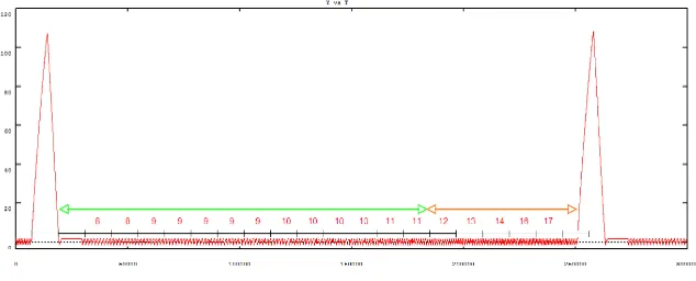
account accurately for this control, we have to fully understand the sequence of bifurcations corresponding to the different phases of GnRH secretion and the occurence of an hysteresis loop. In particular, we have to encompass the rarely investigated case of homoclinic connection occurring in the uncoupled FitzHugh-Nagumo systems when the slope of the slow variable is not steep. There is also a need for good approximations of the period and amplitude of the limit cycle of the regulating system, in the framework of singular perturbation theory (when ε is small but non zero). Hence, the goal of current work is to go on investigating the model behaviour, with the definite aim of constraining the model GnRH output with respect to a physiologically relevant list of specifications (see an instance of GnRH output in Figure 7). These specifications deal with the duration of the luteal (progesterone-dominated) and follicular (estradiol-dominated) phases of the ovarian cycle, and the ratios between (i) the surge duration and the whole cycle duration, (ii) the pulse amplitude and the surge amplitude, and (iii) the increase in pulse frequency from the luteal to the follicular phase. Basing on pure dynamical considerations, we have proposed an algorithm-like procedure to tune the model parameters subject to biologically-meaningful specifications [11].

Figure 7. GnRH secretion pattern along an ovarian cycle: y(t) signal. The great amplitude peaks correspond to the GnRH surge. They are separated by pulses of increasing frequency (the number of peaks between two consecutive ticks are precised). The green double way arrow spans the luteal phase, while the orange one spans the follicular phase (Courtesy of A. Vidal).

From a more generic dynamical viewpoint, this study indirectly addresses the questions of tracking homoclinic connections, where classical Canard cycles disappear, and Bogdanov-Takens like bifurcations of Relaxation Oscillators that occur on a parameter control manifold. Future work will also focus on determining whether the whole system admits a strictly periodic attractive orbit. It is a challenging question dealing with the synchronisation of weakly coupled oscillators and delay to bifurcation analysis.

3.

Appendix

3.1.

Link between backwards reachable sets and Hamilton-Jacobi equations

Let us consider the controlled dynamics described by system (5), wheref is a Lipschitz continuous function, so that there is a unique continuous solution for any measurable u(t).

Given a closed target set M ∈Rn _{and two times τ and t}

1, the solvability setW(τ, t1,M) is the set of states x∈Rn _{such that there exist control functionsuwith values in the compact set U that steer system (5) from}

the statex(U;τ) =xtox(U;t1)∈ M[22]. W(τ, t1,M) can be computed by solving the following optimisation

problem where dσ(x, X) is the signed distance from pointxto setX:

dσu(t, t1;x,M) = min

u∈U{dσ(x(U;t1),M)|x(τ) =x}, W(τ, t1,M) ={x|dσu(t, t1;x,M) = 0} (8)

with dσ(x,M) =

d(x, ∂M) forx /∈ M

The solution of this optimal control problem can be found by solving the following backward HJB equations, whereHf(DxV, x) = min

u∈U{(DxV)

T_{.f(t, x, u)} is the Hamiltonian [5]:}

Vt+Hf(DxV, x) = 0, t≤t1, V(t1, x) =dσ(x,M) (9)

Then the following property is true [22]:

W(τ, t1,M) ={x|V(τ, x) = 0} (10)

Now, the backward reachable set is the set of states from which it is possible to reach the target in at most (t1−t) [19]:

G(t ;t1,M) =

[

t≤s≤t1

W(t, s,M), t≤t1. (11)

This set can also be characterised in the same manner as in expression (10). It is the zero sublevel set of theV

function solution of the HJB equation:

Vt+ min(0, Hf(DxV, x)) = 0, t≤t1, V(t1, x) =dσ(x,M) (12)

G(t ;t1,M) = {x∈Rn|V(t, x) = 0} (13)

References

[1] D.S. Bale, R.J. LeVeque, S. Mitran, and J.A. Rossmanith. A wave propagation method for conservation laws and balance laws with spatially varying flux functions.SIAM J. Sci. Comput., 24(3):955–978, 2003.

[2] S. Ben Said, D. Lomet, D. Chesneau, L. Lardic, S. Canepa, D. Guillaume, C. Briant, C. Fabre-Nys, and A. Caraty. Differential Estradiol Requirement for the Induction of Estrus Behavior and the Luteinizing Hormone Surge in Two Breeds of Sheep.Biol. Reprod., 76(4):673–680, 2007.

[3] M.J. Berger and R.J. LeVeque. Adaptive mesh refinement using wave-propagation algorithms for hyperbolic systems. SIAM J. Numer. Anal., 35(6):2298–2316, 1998.

[4] A. Borisyuk and J. Rinzel. Understanding neuronal dynamics by geometrical dissection of minimal models. In C. Chow, B. Gutkin, D. Hansel, and C. Meunier, editors,Methods and Models in Neurophysics, volume LXXX ofles Houches Summer School, pages 19–72. Elsevier, 2004.

[5] A.E. Bryson and Y.-C. Ho.Applied optimal control. Hemisphere, Washington DC, (1975).

[6] F. Cl´ement and J.-P. Fran¸coise. Mathematical modeling of the GnRH-pulse and surge generator. SIAM J. Appl. Dyn. Syst., 6:441–456, 2007.

[7] F. Cl´ement, M.-A.Gruet, P. Monget, M. Terqui, E. Jolivet, and D. Monniaux. Growth kinetics of the granulosa cell population in ovarian follicles: an approach by mathematical modelling.Cell Prolif., 30:255–570, 1997.

[8] N. Echenim. Mod´elisation et contrˆole multi-´echelles du processus de s´election des follicules ovulatoires. PhD thesis, Paris 11 University, 2006.

[9] N. Echenim, F. Cl´ement, and M. Sorine. Multi-scale modeling of follicular ovulation as a reachability problem. Multiscale Model. Simul., 6:895–912, 2007.

[10] N. Echenim, D. Monniaux, M. Sorine, and F. Cl´ement. Multi-scale modeling of the follicle selection process in the ovary.Math. Biosci., 198:57–79, 2005.

[11] F. Cl´ement and A. Vidal. Bifurcation-based parameter tuning in a model of the GnRH pulse and surge generator, http://www.citebase.org/abstract?id=oai:arxiv.org:0809.1722, 2008.

[12] K.M. Henderson, K.P. McNatty, L.E. O’Keeffe, S. Lun, D.A. Heath, and M.D. Prisk. Differences in gonadotrophin-stimulated cyclic AMP production by granulosa cells from booroola x merino ewes which were homozygous, heterozygous or non-carriers of a fecundity gene influencing their ovulation rate.J. Reprod. Fertil., 81:395–402, 1987.

[13] A.E. Herbison. Multimodal influence of estrogen upon gonadotropin-releasing hormone neurons. Endocr. Rev., 19:302–330, 1998.

[15] R.B. Land. The sensitivity of the ovulation rate of finnish landrace and blackface ewes to exogenous oestrogen. J. Reprod. Fertil., 48:217–218, 1976.

[16] R.J. LeVeque. Wave propagation algorithms for multidimensional hyperbolic systems.J. Comput. Phys., 131(2):327–353, 1997. [17] P. Michel. A singular asymptotic behavior of a transport equation.C. R. Math. Acad. Sci. Paris, 346:155–159, 2008. [18] I. Mitchell. The flexible, extensible and efficient toolbox of level set methods.J. Sci. Comput., 35:300–329, 2008.

[19] I. Mitchell, A.M. Bayen, and C.J. Tomlin. A time-dependent Hamilton-Jacobi formulation of reachable sets for continuous dynamic games.IEEE Trans. Automat. Control, 50:947–957, 2005.

[20] L. Perko.Differential equations and dynamical systems. Springer, 2000.

[21] C. Pisselet, F. Cl´ement, and D. Monniaux. Fraction of proliferating cells in granulosa during terminal follicular development in high and low prolific sheep breeds.Reprod. Nutr. Dev., 40:295–304, 2000.