Minimizing Time Delay of Information Routed Across Dynamic Temporal Sensor Networks

www.astesj.com

Special Issue on Multidisciplinary Sciences and Engineering

Minimizing Time Delay of Information Routed Across Dynamic

Temporal Sensor Networks

Michael J. Hirsch*,1, Azar Sadeghnejad2

1_{ISEA TEK, LLC, 32751, U.S.A.}

2_{Radiation-Oncology Department, University of Texas - Southwestern Medical Center, 75390, U.S.A.}

A R T I C L E I N F O A B S T R A C T

Article history:

Received: 13 July, 2018 Accepted: 10 August, 2018 Online: 20 August, 2018

Keywords:

Information Routing Sensor Network

Communication Topology

In this research we address the problem of routing information across dynamic temporal sensor networks. The goal is to determine which in-formation, generated by sensors on resources at various times, is able to be routed to other resources, consumer resources, within the given infor-mation time window, while being constrained by temporally dynamic bandwidth limitations across the sensor network, and storage limitations on the resources. A mathematical model of the problem is derived, and used to find solutions to the problem. In addition, a heuristic is developed to efficiently find good quality solutions. Monte-Carlo simulations are performed comparing solutions found by commercial software with the heuristic.

1

Introduction

This paper is an extension of work originally presented at the Military Communications Conference [1]. Wire-less sensor networks are a class of networks in which some or all of the sensors or resources collect, ana-lyze, and communicate data acquired from their en-vironment (external or internal) to other nodes in the network [2]. These other nodes could be resources, sensors, or fixed or mobile command posts. Mobile ad-hoc networks (MANETs) are a subset of wireless sensor networks that have an absence of a fixed infrastruc-ture, and exhibit a dynamic communication topology [3]. Resources within transmission range of others communicate directly (depending on bandwidth limi-tations) and cooperation among intermediate resources is required for resources to communicate with others outside of their direct communication range. More and more networks, in both the military and commercial domain, are relying on wireless sensor networks and MANETs [4, 5, 6].

The ability for data to be collected by manned and unmanned vehicles engaged in military, government, and commercial missions is increasing at an exponen-tial rate [7]. Examples include high-resolution video, telephone intercepts, traffic congestion reports, inter-nal vehicle system states, among others. In commer-cial telecommunication networks, there are instances where the capacity across the network is in the

ter-abytes per second range [8]. Networks of this type have the ability to transmit all data that is collected with-out restrictions or delays. However, in times of crisis and disaster, commercial and civil communication net-works can be severely degraded [9, 10]. And in military missions, bandwidth is oftentimes severely limited, which results in a reduction in transmission and shar-ing of information that can be mission-critical. And this will continue to be the case due to the rise of op-erations performed in anti-access/area denial (A2AD) environments, against near-peer adversaries. In the past, this meant that information collected by vehicles would not be processed, analyzed, and understood un-til after the vehicle had returned to base and ‘uploaded’ all of the collections [7, 11].

In performing more of the processing and analysis on-board the vehicles, there has the potential for less bandwidth requirements for vehicles to share informa-tion important for mission success. In effect, this can be seen aspushing the smarts out to the tactical edge.

Each generation of manned and unmanned vehicles is having more and more processing capabilities on-board [11]. Examples include internally monitoring on-board systems, fusing information collected from various on-board sensors, picking out a person of inter-est from a full motion video, and deciding how much information should be sent over the sensor network and to whom should be the recipient of such informa-tion [12]. While some of the collected informainforma-tion can

*_{Michael J. Hirsch, ISEA TEK, 620 N. Wymore Rd., Ste. 260, Maitland, FL 32751 U.S.A., [email protected]}

just be generated and stored on a vehicle, and offloaded upon mission completion, other generated information is vital to mission success, and must be transmitted to control station(s) or other resources during mission execution.

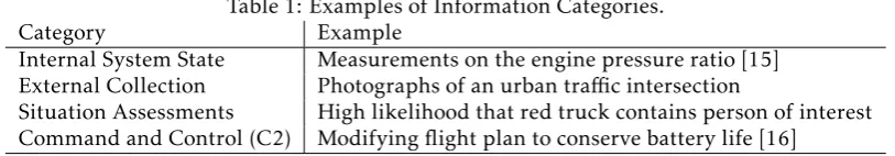
To address this, we consider the following problem. There are a set of resources (moving or fixed) that have a set of Information Generation Requests (IGRs) to sat-isfy over a given time horizon. If a resource executes a task to perform the IGR, then an associated piece of information is generated. We will use the term IGR to denote the information that gets generated. Each IGR can come from one of a fixed set of categories (for an example of information categories, see Table 1). In addition, each IGR has associated with it the following characteristics: an expected time of generation, the set of consumer resources (those resources that would find this information important for their mission), the time by which the information needs to be delivered to the to be of use, the expected original size of the information, and the priority of the information (i.e., a measure of its importance in the mission). We note that the priority of an IGR could be determineda priori

(e.g., information collected about one kinematic loca-tion is deemed very important and therefore is given a high priority) or dynamically on-board the resource at the time of collection, if the resource has the ap-propriate analytics (e.g., image is given low priority because it does not contain any red cars). By a ‘con-sumer resource’ for a particular IGR, we mean that the resource actually performs some processing with that information (e.g., fuses that information with other information [13, 14], makes command and control de-cisions, etc.).

There is a dynamic sensor network topology in place over the time horizon. This dynamic network has finite, but varying bandwidth limitations between any two resources at any given time, and in many cases there might not be a direct connection between two resources. Each IGR can be sent over the network with different potential granularities (e.g., 100% of original size, 70% of original size, etc.), but there is a minimum size percentage with which the information remains useful to the consumer of the information. As an IGR gets routed from the generating resource to the con-sumer resource, all resources along this route will need to store this IGR locally for some amount of time. The generating resource will need to store an IGR from the time of generation until the IGR is completely sent to the next resource in the path to the consumer re-source(s). Non-consumer resources along this path will need to store the IGR from the time the resource begins receiving the IGR until the time the resource has com-pletely transmitted the IGR to the next resource along the path. And the consumer resource(s) will need to store the IGR form the time they begin receiving it until at least they have finished processing the IGR.

Each resource has a finite storage capacity, and re-sources can triage information they have stored (e.g., once a piece of information is generated and com-pletely sent to the next resource along the path to the

consumer, the generator resource can delete the infor-mation from storage). The objective is then to deter-mine which IGRs to route over the network, how to route those IGRs so that they have a minimal time de-lay (difference between time of consumption and time of generation), from generating resource to consumer resource over the time horizon, while also attempt-ing to maximize the size of granularity of each IGR that is routed. In turn, this produces the higher-level end product of determining which IGRs should be ac-complished for mission objectives, given the network topology characteristics.

There has been some prior research into routing schemes for collected data across a dynamic network. In [17], the author considered the problem of sinkholes in a network. A sinkhole node attempts to deceive all the nodes in the network to route network traffic to the sinkhole, by broadcasting false routing informa-tion across the network. An approach based upon secondary caching was developed to prevent a sink-hole attack in dynamic source routing sensor networks. In [18], the author consider cellular data networks and the significant increase in data being transmitted over these networks. Their research looked at data traffic management techniques, whereby users and au-tomated approaches ‘flag’ messages that are of low priority, and an higher-level agent-based scheduling system had the ability to delay scheduling of low pri-ority messages during peak load times. In [19], the authors considered the problem of extending lifetimes of wireless sensor networks. In their view, the sending of redundant data across sensor networks reduced the lifetime of these networks. They looked at providing certain nodes in the network to function as ‘data ag-gregation’ nodes, receiving collected data from other nodes in the network, fusing or aggregating the data to-gether to reduce redundant information, and then pass-ing this reduced set of data onwards to a base station. They employed a grid-based routing and aggregator selection scheme to find the minimum number of ag-gregation points while routing data to the base station ensuring that the network lifetime is maximized.

Table 1: Examples of Information Categories.

Category Example

Internal System State Measurements on the engine pressure ratio [15] External Collection Photographs of an urban traffic intersection

Situation Assessments High likelihood that red truck contains person of interest Command and Control (C2) Modifying flight plan to conserve battery life [16]

acoustic networks and the long propagation delays and low bandwidths inherent in such networks. A set of nodes was using the same bandwidth channel, and because their problem had bursty data, the so-lution approach looked at submitting their requests randomly, as demand dictated. A medium access con-trol protocol was in place to minimize the number of collisions among the information flowing across the network. In [24], the researchers investigated ways to enhance the operations of a power grid. One of the ways, taking advantage of the high sampling rates of the measurement data, required a high bandwidth, net-worked communication system. Their results derived a method to simulate, design, and test the adequacy of a communication system for a particular grid layout.

The rest of this paper is organized as follows. In Sec-tion 2, we introduce the parameters and decision vari-ables for our model, and rigorously derive the mathe-matical program representing our problem. Section 3 develops a heuristic to efficiently find good quality so-lutions. Section 4 analyzes the results of computational experiments performed on various scenarios, compar-ing commercial software solvcompar-ing a linearized version of the mathematical program and the solutions found by the heuristic. Section 5 provides some concluding remarks and future research directions.

2

Mathematical Formulation

In this section, we rigorously derive mathematical equations to model the problem of interest. This re-sults in a mixed-integer nonlinear program (MINLP). We note that the time dimension in the model is dis-cretized, over the planning horizon ofK_time-steps.

2.1

Parameters

This section lists the parameters for the mathematical programming problem.

I _{is the set of resources,i, i1, i2,}∈ I_;

J _{is the number of Information Generation}

Re-quests (IGR)s,j∈ {_{1, . . . ,}J }_;

K _{is the number of time-steps in the planning}

horizon,k,kˆ∈ {_{1, . . . ,}K}_;

Pmin_{is the minimum percentage an IGR can be} decreased in size and still be considered useful to consumer resource(s);

τi,jis the number of time-steps after a consumer receives an IGR before the consumer can delete

the IGR, i.e., the number of time-steps it takes resourcei(the consumer resource) to ‘process’ IGRj;

ρjis the expected priority of IGRj;

S_jois the expected original size of IGRj;

gj is the expected time of generation of IGRj;

dj is the time by which IGRjis due to the con-sumer resource(s) of the IGR;

Gi,j=

      

1 if resourceiis tasked with generating IGRj

0 o.w. ;

Ci,j=

      

1 if resourceiis a consumer of IGRj

0 o.w. ;

Liis the storage capacity of resourcei;

bi1,i2,kis the expected bandwidth capacity from

resourcei1to resourcei2at time-stepk;

¯

ρ is the largest expected priority, i.e., ¯ρ = max

j

h

ρj

i

;

ωd andωsare the weighting coefficients for the priority and size components of the objective function;

M_{is a large enough constant, used in Constraints}

(7).

2.2

Variables

This section lists the decision variables for the mathe-matical programming problem.

xj=

              

1 if IGRjis chosen to be routed from the generating resource to the consumer resource(s) 0 o.w.

, ∀_j;

sj = the size of IGR j sent to the consumer re-source(s), ∀_j;

ai1,i2,j,k= the amount (size) of IGRj sent from

resource i1 to resource i2 during time-step

k, ∀_{i1, i2(,i1), j, k;}

αi1,i2,j,k=

          

1 if resourcei1sends some of IGRj

to resourcei2during time-stepk

0 o.w.

,

mi,j,k= the amount of IGRjbeing stored on re-sourceiat time-stepk, ∀_{i, j, k.N.B.: For}

consis-tency of the constraints,mi,j,0= 0 ∀i, j;

φi1,i2,j=

          

1 if resourcei1is assigned to send

IGRjto resourcei2

0 o.w.

,

∀_{i1, i2(,i1), j;}

βi,j= the amount of time resourceitakes in send-ing IGR j to other resources, i.e., the time be-tween resourceicompletely receiving or generat-ing IGRjto the time where resourceino longer needs IGRj, ∀_{i, j;}

ti,j,k=

              

1 if resourceicumulatively receives (or generates)sjsize units of IGRjat time-stepk

0 o.w.

,

∀_{i, j, k;}

Ti,j = the time-step at which resource i com-pletely receives (or generates) IGRj, ∀_{i, j;}

di,j,k=

          

1 if resourceideletes IGRjfrom storage at time-stepk

0 o.w.

,

∀_{i, j, k;}

Di,j= the time-step at which resourceideletes IGRjfrom its storage, ∀_{i, j;}

Qi,j = the time at which resourcei completely consumes (or transmits) IGRj, ∀_{i, j;}

ei,j,k=

          

1 if resourceireceives (or generates) IGRjby time-stepk

0 o.w.

,

∀_{i, j, k.}

N.B.: For consistency of the constraints, it is necessary to setei,j,0 = 0 ∀i, j. Also, note that

ei,j,k= 1 implies thatei,j,`= 1 for each` > kand

ei,j,k= 0 implies thatei,j,`= 0 for each` < k.

2.3

Nonlinear Mathematical Formulation

This section presents the mathematical model of the problem described in Section 1, resulting in a mixed-integer nonlinear program (MINLP).

max ωd·

             J X j=1 X

i∈I_: Ci,j=1

K_+gj·_xj−_Ti,j K             

+ωs·

        J X j=1 sj

S_jo

        (1) s.t.

sj≤Sjo·xj ∀j (2)

sj≥ Pmin·Sjo·xj ∀j (3)

X

j

mi,j,k≤Li ∀i, k (4)

mi,j,k=mi,j,k−₁+ X

i1∈I

ii,i

ai1,i,j,k

−_di,j,k·_sj+δh_gj−_ki·_Gi,j·_sj ∀_{i, j, k (5)}

K X

k=1

αi1,i2,j,k≤ K ·xj ∀i1, i2, j (6)

M ·_αi

1,i2,j,k≥ai1,i2,j,k ∀i1, i2, j, k (7)

X

j

ai1,i2,j,k≤bi1,i2,k ∀i1, i2, k (8)

gj X

k=1

ai1,i2,j,k= 0 ∀i1, i2, j (9)

K X

k=1

ai1,i2,j,k≤sj ∀i1, i2, j (10)

ei,j,k>

X

i1∈I

i1,i k

X

ˆ

k=1

a_i

1,i,j,kˆ

−_sj−₁−_xj ∀_k, ∀_{i, js.t.Gi,j= 0 (11)}

ei,j,k·sj

≤X

i1∈I

i1,i k

X

ˆ

k=1

a_i

1,i,j,kˆ ∀k, ∀i, js.t.Gi,j= 0 (12)

ti,j,k≥ei,j,k−ei,j,k−₁ ∀i, j, k (13)

K X

k=1

ti,j,k≤xj ∀i, j (14)

ti,j,gj=xj ∀i, js.t.Gi,j= 1 (15)

Ti,j=

K X

k=1

k·_ti,j,k ∀_{i, j (16)}

Ti,j≤dj·xj ∀i, j (17)

Qi,j=Ti,j+τi,j·xj ∀i, js.t.Ci,j= 1 (18)

Qi,j=Ti,j+βi,j ∀i, js.t.Ci,j= 0 (19)

βi1,j≥k·αi1,i2,j,k−Ti1,j ∀i1, i2, j, k (20)

Di,j> Qi,j−

       1− K X k=1 ti,j,k       

Di,j=

K X

k=1

k·_di,j,k ∀_{i, j (22)}

K X

k=1

di,j,k≤xj ∀i, j (23)

X

i1∈I

i1,i

φi1,i,j≤xj ∀i, j (24)

K X

k=1

αi1,i2,j,k≤ K ·φi1,i2,j ∀i1, i2, j (25)

K X

k=1

αi1,i2,j,k≥φi1,i2,j ∀i1, i2, j (26)

X

i2∈I

i2,i

αi,i2,j,k≤

k−₁ X

ˆ

k=1

t_i,j,kˆ ∀i, j, k (27)

sj=

K X

k=1 X

i1∈I

i₁,cj

ai1,cj,j,k ∀j (28)

K X

k=1 X

i2∈I

αcj,i2,j,k= 0 ∀j (29)

xj, αi1,i2,j,k, φi1,i2,j, ti,j,k, di,j,k, ei,j,k∈ {0,1}

∀_{i, i1, i2, j, k (30)}

sj, ai1,i2,j,k, mi,j,k∈

h

0, S_joi ∀_{i, i1, i2, j, k (31)}

βi,j, Di,j, Ti,j, Qi,j∈[0,K]∩Z ∀i, j, k (32)

2.4

Interpretation of Nonlinear

Mathe-matical Formulation

In this section, we explain the objective function and each of the constraints that are part of the mathemati-cal formulation.

• The objective function, Equation (1), is a weighted combination of the time delay and size of the IGRs routed across the network.

The first term in the objective function deals with the time delay of those IGRs chosen to be routed. The sum is over all IGRs j and all resources i

that are consumers of IGRj(i.e., those resources such that the parameterCi,j= 1). When an IGR

jis not chosen to be routed,xjis set to be 0 and

Ti,j also ends up as 0, so this term is 0. When an IGR is chosen to be routed,xj is set to be 1 andTi,j is set to be the time at which resource

i completely receives IGRj. The time IGRj is generated is given by the parametergj. The max-imum value of this term is 1, which occurs when

Ti,j=gj (which is an idealistic situation), while the minimum value of this term is K+gKj−dj, which

can be 0 whengjis 0 anddjisK.

The second term of the objective function deals with the size of the IGRs chosen to be routed,

looking at the ratio of the actual size of the IGR that gets routed versus the original size.

Note that that scale of these two terms are the same, i.e., they are both within [0,1], and are unit-less. The first term is weighted byωd, while the second term is weighted byωs.

• Constraints (2) forcesjto be less than or equal to

S_joif IGRjis chosen to be routed, and 0 if IGRj

is not chosen to be routed;

• Constraints (3) requiresj to be greater than or equal to the minimal amount to be routed for IGRj(Pmin·_So

j), if IGRjis chosen to be routed; • Constraints (4) ensure that at each time-step, the storage capacity for each resource is not ex-ceeded;

• Constraints (5) determine the amount of IGR

j stored on resource iat time kas the amount stored at timek−_{1 plus the amount sent to}

re-sourceiat time-stepkminussjif IGRjis deleted from resourcei’s storage at time-stepk, plussjif IGRjis chosen to be routed by resourceiand is generated at time-stepk.N.B.: The Dirac-Delta impulse functionδ[q] returns 1 whenq= 0 and returns 0 otherwise [25];

• Constraints (6) only allowαi1,i2,j,kto be greater

than 0 if IGRjis chosen to be routed;

• Constraints (7) forceai1,i2,j,kto be 0 if resourcei1

is not sending IGRjto resourcei2at time-stepk;

• Constraints (8) limit the amount of information traveling from resourcei1toi2at time-stepkto

be no more that the capacity of this edge,bi1,i2,k;

• Constraints (9) enforce that no resource can send IGRjbefore it is generated;

• Constraints (10) enforce that resourcei1send no

more thansjof IGRjto resourcei2;

• For those resources that do not generate IGRj

and IGR j is chosen to be routed, Constraints (11) forceei,j,kto be 1 if allsjof IGRjreaches re-sourceiat or before time-stepk. This constraint allowsei,j,kto be 0 or 1 otherwise;

• For those resources that do not generate IGRj, Constraints (12) forceei,j,kto be 0 while not allsj of IGRjhas reached resourcei. This constraint allowsei,j,kto be 0 or 1 otherwise;

• Constraints (13) setti,j,kto be 1 at the time-step that resourceireceives allsjof IGRj, and to be 0 for all other time-steps;

• Constraints (14) enforce that resourcei can re-ceive IGRjat most once;

• Constraints (16) setTi,j to be the time at which resourceireceives IGRj;

• Constraints (17) enforce that any resource that re-ceives IGRj, must do so before its due date/time, if IGRjis chosen to be routed;

• Constraints (18) define the time at which re-sourceihas completely ‘processed’ IGRj, if re-source i is a consumer of IGR j and IGR j is chosen to be routed;

• Constraints (19) define the time at which re-source i has completely transmitted IGR j to other resources, if resourceiis not a consumer of IGRjand IGRjis chosen to be routed;

• Constraints (20) determine the amount of time it takes resourceito send IGRjto other resources, once resourceireceives or generates IGRj;

• Constraints (21) ensure that if IGRj is chosen to be routed, that IGRjcannot be deleted from resource iuntil resourcei is finished with the IGR;

• Constraints (22) determine the time at which re-sourceideletes IGRj;

• Constraints (23) ensure that resourceican delete IGRjat most once;

• Constraints (24) enforce that at most one re-source is assigned to send IGRjto resourcei;

• Constraints (25) only allow resourcei1to send

IGRjto resourcei2if it is assigned to;

• Constraints (26) forcei1to send IGRjto resource

i2during at least one time-step, ifi1is assigned

to send IGRjto resourcei2;

• Constraints (27) does not allow resourceito send any portion of IGRjat time-stepkif resourcei

has not completely received (or generated) IGRj

by time-stepk−_1;

• Constraints (28) ensure that the consumer re-source(s) of IGRjreceives allsjunits, if IGRjis chosen to be routed;

• Constraints (29) prohibit resourcecj (the con-sumer of IGR j) from sending IGRj to other resources;

• Constraints (30) – (32) are domain restriction constraints on the decision variables.

3

Solution Methodologies

The formulation derived in Section 2.3 is a nonlinear mixed-integer programming problem. However, this formulation can be linearized through standard tech-niques from operations research [26], resulting in a

mixed-integer linear program (MILP). As such, in the-ory the MILP formulation could be solved using a num-ber of commercial software packages (e.g.,CPLEX[27],

LINDO[28], etc.). It can be shown that this optimization

problem isNP-Hard, as a variant of the vehicle rout-ing problem with split deliveries and time windows [29, 30, 31], which necessitate heuristic strategies for finding good-quality solutions efficiently [32, 33] when the problem instances are of sufficient size.

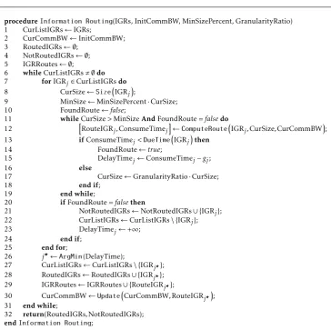
The heuristic developed is split into two phases, an Information Routing phase, and a Storage Manage-ment phase. The Information Routing phase attempts to route all of the IGRs, from generating resource to consuming resource(s), without consideration of stor-age limitations on the individual resources. The only constraints taken into account in the Information Rout-ing phase are the bandwidth limitations across the sensor network. The Storage Management phase of the heuristic then factors in the storage limitations of each resource to reduce the solution to one that is feasible.

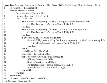
Figures 2 and 1 provide pseudo-code for the In-formation Routing and Storage Management phases, respectively. The Information Routing function is in-put the set of IGRs (and all information about the IGRs), the initial allocation of bandwidth across the network over time (InitCommBW), the minimum per-centage (in size) an IGR is able to be reduced and still be useful (MinSizePercent), and the ratio by which to reduce the size of the IGR in sending over the network, if needed (GranularityRatio). Lines 1 to 5 initialize internal variables. Lines 6 to 32 get executed while there are still IGRs on the list to be routed. For each IGR still on the CurListIGRs list, lines 7 to 25 attempt to determine a route for the IGR that allows for at least the minimum size for the IGR to be routed. Line 8 com-putes the size of the current IGR and line 9 comcom-putes the minimal allowable size of the IGR to be routed. While a feasible route for the current IGR has not been found, and the current size of the IGR is larger then the minimum allowable size, lines 11 to 19 get exe-cuted. Line 11 calls the functionComputeRoute, given the current size of the IGR and the current allocation of bandwidth across the network. Returned from this function are the route for this IGR from generating resource to consumer resource, as well as the time the IGR will completely reach the consumer resource. If the time by which the consumer completely receives the IGR is less than the due date of the IGR, then a potential route for this IGR is found, and the potential time delay for this IGR is computed. Otherwise, the size of the IGR is reduced by the granularity ratio. If a potential route is not found in lines 11 to 19, then this IGR is moved to the NotRoutedIGRs list and removed from the current list of IGRs (lines 21 and 22). Line 23 also sets this IGR to have a delay time of +∞_{. After}

procedureStorage Management(ResourceList, RoutedIGRs, NotRoutedIGRs, MaxStorageSize) 1 CurrentRL←_{ResourceList;}

2 whileCurrentRL,∅do

3 CurR←Choose(CurrentRL);

4 CurrentRL←_CurrentRL\_CurR; 5 fork= 0toKdo

6 foreach IGR`completely transited through CurR by time-stepkdo

7 CurR←RemoveFromStorage(CurR,IGR`, k,K);

8 end for;

9 foreach IGR`completely consumed by CurR by time-stepkdo

10 CurR←_{RemoveFromStorage(CurR,IGR`, k,}K_);

11 end for;

12 ifStorage(CurR, k)>MaxStoragethen

13 foreach IGR`generated by CurR and completely transited by time-stepkdo

14 CurR←_{RemoveFromStorage(CurR,IGR`, k,}K_);

15 end for;

16 end if;

17 ListIGRs←GetIGRs(CurR, k); 18 SortIGRs←Sort(ListIGRs);

19 whileStorage(CurR, k)>MaxStoragedo

20 IGR`←Choose(SortIGRs);

21 RemoveFromRouting(IGR_`);

22 NotRoutedIGRs←_{NotRoutedIGRs}∪ {_{IGR`</sub>}<sub>;</sub> 23 RoutedIGRs←<sub>RoutedIGRs</sub>\ {<sub>IGR`}}_;

24 end while;

25 end for;

26 end while;

27 return(RoutedIGRs,NotRoutedIGRs);

endStorage Management;

Figure 1: Pseudo-code for the Storage Management phase of the heuristic.

Table 2: Categories, and values used for the number of resources and density over the numerical experiments.

Category N Density

Extra Small 3

Small 4,5,6 1,0.67,0.33 Medium 8,10,12

Large 15,20,25

saved into the set IGRRoutes in line 29, and the cur-rent bandwidth allocation across the temporal network is updated (due to this IGR having its route finalized) in line 30. This process in lines 6 through 32 continues until the set CurListIGRs is empty. The output from the Information Routing function is the set of IGRs that have been routed (along with all of the necessary details of the routes), as well as the set of IGRs not able to be routed.

The Storage Management function takes as input the list of resources, the list of routed IGRs, the list of IGRs that are not able to be routed, and the maximum storage size for each resource. While not all of the resources have been considered, lines 2 through 26 are executed. Line 3 chooses a resource from those still to be considered. Lines 5 to 25 get executed for each time-step of the time horizon. In lines 6 to 8, each IGR that has completely transited through the current resource by the time-step under consideration, gets re-moved from the resources’ storage, from the time-step under consideration to the end of the time horizon. In lines 9 to 11, each IGR that has been completely consumed by the current resource, by the time-step under consideration, gets removed from the resources’

procedureInformation Routing(IGRs, InitCommBW, MinSizePercent, GranularityRatio) 1 CurListIGRs←_IGRs;

2 CurCommBW←_InitCommBW; 3 RoutedIGRs← ∅_;

4 NotRoutedIGRs← ∅_; 5 IGRRoutes← ∅_;

6 whileCurListIGRs,∅do 7 forIGRj∈CurListIGRsdo

8 CurSize←SizeIGRj

;

9 MinSize←_{MinSizePercent}·_CurSize;

10 FoundRoute←_false;

11 whileCurSize>MinSizeAndFoundRoute =falsedo

12 hRouteIGRj,ConsumeTimej

i

←ComputeRouteIGRj,CurSize,CurCommBW

; 13 ifConsumeTimej<DueTimeIGRj

then

14 FoundRoute←_true;

15 DelayTime_j←ConsumeTimej−gj;

16 else

17 CurSize←_{GranularityRatio}·_CurSize;

18 end if;

19 end while;

20 ifFoundRoute =falsethen

21 NotRoutedIGRs←_{NotRoutedIGRs}∪ {_IGRj}_; 22 CurListIGRs←_CurListIGRs\ {_IGRj}_;

23 DelayTime_j←₊∞_;

24 end if;

25 end for;

26 j?←ArgMin(DelayTime);

27 CurListIGRs←_CurListIGRs\ {_IGR

j?}; 28 RoutedIGRs←_RoutedIGRs∪ {_IGR

j?}; 29 IGRRoutes←_IGRRoutes∪ {_RouteIGR

j?};

30 CurCommBW←UpdateCurCommBW,RouteIGR_j?

; 31 end while;

32 return(RoutedIGRs,NotRoutedIGRs);

endInformation Routing;

Figure 2: Pseudo-code for the Information Routing phase of the heuristic.

4

Computational Experiments

4.1

Test Environment

Java jdk 1.8.0 25 was used to code up the heuristic, the actual exact MILP, and the generation of scenario data. CPLEX Optimization Studio V12.6.3 [27] was called to solve the exact MILP.Matlab R2011b (7.13.0.564) [34] was used to generate combinations of input pa-rameters, as well as to analyze the results of all ex-periments. All experiments were conducted on a Dell Precision Tower 7810 with an Intel(R) Xeon(R) CPU E5-2630 v3 @2.40GHz 2.40 GHz with 32.0 GB memory.

4.2

Experimental Results

The aim of our experiments were to investigate the so-lution quality found by the heuristic, as compared with commercial software, as well as to determine how close to optimal were the solutions found by the heuristic. We used the commercial software CPLEX [27] to solve the linearized formulation of the mathematical model presented in Section 2. However, as can be seen from the results that follow, for some of the scenarios CPLEX was not able to find solutions significantly close to op-timal, within the time-limits to find a solution. Thus, we also ran CPLEX to solve the linearized formula-tion, providing CPLEX an initial solution found from

running the heuristic. These two sets of experiments involving CPLEX are described as ‘‘CPLEX w/o Init. Soln.’’ and ‘‘CPLEX w/ Init. Soln.’’, respectively. To test the heuristic, as well as CPLEX, we created numer-ous scenarios, varying the number of resources (N) and the density of the underlying communication network topology, as displayed in Table 2.

Table 3: Parameter categories and values used for the numerical experiments. For those parameters with only a minimum value, that is the fixed value for the parameter. For those parameters that have a minimum and maximum value, the distribution listed is the probability distribution through which a specific parameter is determined, via a random draw.

Parameter Min. Value Max. Value Dist.

Number Time-Steps 20

Bandwidth per Directed Edge 0 100 Uniform

per Resource

Number of IGRs in Scenario 5 10 Uniform

per Resource

Time Delay Between IGR 7 20 Uniform

Generation and Consumption

Resources that Neither Generate d_0.2·_Ne

nor Consume IGRs

IGR Size 25 250 Uniform

Storage Capacity 750 1500 Uniform

per Resource

Granularity Ratio 0.9

MinSizePercent 0.8

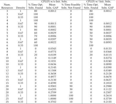
Table 4: Solution quality analysis, according to Equation (34), for the mathematical formulation using CPLEX, without and with an initial input solution.

CPLEX w/o Init. Soln. CPLEX w/ Init. Soln.

Num. % Time Opt. Mean % Time Feasible % Time Opt. Mean

Resources Density Soln. Found Soln. GAP Soln. Not Found Soln. Found Soln. GAP

3 1 80 0.0012 0 80 0.0012

3 0.67 100 0 100

3 0.33 100 0 100

4 1 100 0 100

4 0.67 90 0.0013 0 90 0.0012

4 0.33 90 0.0001 0 90 0.0001

5 1 80 0.0002 0 90 0.0001

5 0.67 60 0.0029 0 50 0.0027

5 0.33 70 0.0006 0 70 0.0006

6 1 60 0.0207 0 50 0.0035

6 0.67 60 0.0022 0 70 0.0093

6 0.33 100 0 100

8 1 0 0.0343 0 0 0.0133

8 0.67 0 0.0775 0 10 0.0368

8 0.33 20 0.0109 0 20 0.0115

10 1 0 0.1149 0 0 0.0274

10 0.67 0 0.1031 0 0 0.0240

10 0.33 0 0.0636 0 0 0.0890

12 1 0 0.2145 0 0 0.0390

12 0.67 0 0.1308 0 0 0.0349

12 0.33 0 0.3658 0 0 0.2128

15 1 0 0.4977 0 0 0.0678

15 0.67 0 0.2130 0 0 0.0637

15 0.33 0 0.4390 10 0 0.1810

20 1 0 0.9583 90 0 0.2988

20 0.67 0 0.6205 30 0 0.1122

20 0.33 0 0.2709 10 0 0.2507

25 1 0 1.0000 100 0 0.2614

25 0.67 0 1.0000 100 0 0.3739

25 0.33 0 0.3702 10 0 0.2155

time-step, due to external environmental conditions (e.g., weather, topography, etc). In addition, this can

Table 5: Average normalized distance, computed according to Equation (35), between the heuristic and CPLEX with/without the initial solution, for those cases where CPLEX found at least a feasible solution. Note: An entry is left blank whenever CPLEX was not able to find a feasible solution for any of the scenarios.

Num. CPLEX w/out CPLEX w/

Resources Density Init Soln Init Soln

3 1 -0.132 -0.132

3 0.67 -0.127 -0.127

3 0.33 -0.115 -0.115

4 1 -0.072 -0.072

4 0.67 -0.174 -0.174

4 0.33 -0.330 -0.330

5 1 -0.098 -0.098

5 0.67 -0.194 -0.194

5 0.33 -0.212 -0.212

6 1 -0.071 -0.089

6 0.67 -0.151 -0.145

6 0.33 -0.481 -0.481

8 1 -0.064 -0.085

8 0.67 -0.079 -0.128

8 0.33 -0.400 -0.400

10 1 0.024 -0.071

10 0.67 -0.013 -0.120

10 0.33 -0.281 -0.254

12 1 0.158 -0.066

12 0.67 0.070 -0.100

12 0.33 0.300 -0.102

15 1 0.779 -0.051

15 0.67 0.090 -0.086

15 0.33 0.491 -0.114

20 1 1.186 -0.037

20 0.67 0.536 -0.066

20 0.33 -0.068 -0.108

25 1 -0.035

25 0.67 -0.036

25 0.33 0.109 -0.104

connecting it to other nodes.

Density = |E|

|_N| ·₍|_N| −₁₎ (33)

For each combination of number of resources and density, 10 Monte-Carlo scenarios were created ran-domly. For each scenario generated, the remaining pa-rameters were derived from the information in Table 3, and then kept fixed for the scenario. In addition, the coefficients of the two terms in the objective function (time-delay and size),ωd andωs, were fixed to 0.7 and 0.3 for all scenarios. Each approach (‘‘CPLEX w/o Init. Soln.’’, ‘‘CPLEX w/ Init. Soln.’’, and the heuristic) were given 900 seconds to solve each scenario instance. For those cases where CPLEX did not solve the problem to optimality within the 900 seconds, the best solution found by CPLEX is considered. We note that there are cases in the tables to follow where CPLEX was not able to find even a feasible solution by the time-limit, hinting at the limitations of commercial software as the size of the problems get large.

Table 4 examines the results just from the exact approach, using CPLEX (without and with an initial

Table 6: Mean Time Delay between generation and consumption of IGRs chosen to be routed, for each solution approach. For those cases where CPLEX is not able to find a feasible solution within the time-limit for any scenarios, the entry is left blank. The results are shown as mean:standard deviation.

Num. CPLEX w/out Heuristic CPLEX w/

Resources Density Init Soln Init Soln

3 1 8.956:0.758 5.070:1.120 8.937:0.738

3 0.67 9.691:1.387 4.968:0.897 9.658:1.389

3 0.33 10.223:0.993 4.651:0.722 10.194:0.960

4 1 9.268:0.954 4.105:0.335 9.278:0.952

4 0.67 9.867:0.734 5.059:0.680 9.856:0.697

4 0.33 10.096:1.153 6.036:1.208 10.128:1.168

5 1 9.004:0.676 3.773:0.327 9.030:0.663

5 0.67 9.762:0.779 5.073:0.433 9.735:0.756

5 0.33 9.588:1.137 5.321:0.700 9.595:1.128

6 1 9.300:0.571 4.021:0.296 9.270:0.582

6 0.67 9.502:0.988 5.257:0.345 9.571:0.953

6 0.33 9.925:1.093 6.361:0.861 9.944:1.050

8 1 9.201:0.700 4.016:0.247 9.186:0.639

8 0.67 9.233:0.558 4.704:0.340 9.426:0.830

8 0.33 10.047:0.665 6.433:0.560 10.099:0.667

10 1 9.010:0.560 3.807:0.321 9.248:0.613

10 0.67 8.504:0.580 4.517:0.316 8.788:0.658

10 0.33 9.460:0.457 6.117:0.519 9.928:0.984

12 1 8.632:0.482 3.846:0.234 9.242:0.494

12 0.67 8.950:0.458 4.684:0.313 9.324:0.497

12 0.33 9.362:0.603 6.194:0.334 11.301:0.979

15 1 7.573:0.398 3.820:0.122 9.599:0.288

15 0.67 8.590:0.698 4.411:0.204 9.197:0.570

15 0.33 9.449:1.149 5.924:0.569 11.035:0.874

20 1 7.633:0.000 3.688:0.148 9.692:0.348

20 0.67 7.586:0.312 4.376:0.068 9.961:0.541

20 0.33 8.684:0.512 5.866:0.269 10.534:1.066

25 1 3.721:0.096 9.629:0.312

25 0.67 4.366:0.211 10.469:0.287

25 0.33 8.471:0.424 5.537:0.139 10.359:1.046

(34), whereubis the upper bound on the solution value andsf is the solution found by CPLEX. We note that when CPLEX finds the optimal solution,ub=sf and theGAP is therefore 0, and when CPLEX is not able to find even a feasible solution, we assigned the trivial solution ofsf = 0 (the worst feasible solution for the model), resulting in aGAP value of 1.

GAP =ub−sf

ub (34)

What is apparent from Columns 4 and 7 of Table 4 is that CPLEX with an initial solution performs better most of the time as compared to CPLEX without an initial solution. In most cases, there is a significant decrease in the mean gap. However, there are a few cases that are counter-intuitive. Specifically when the number of resources is 6, 8, or 10 and the densities are 0.67, 0.33, or 0.33 respectively. For these three combinations, CPLEX without an initial solution has a smaller mean gap than does CPLEX with an initial solution. This is because there was one scenario in each of these combinations where the heuristic found

a solution not close to the optimal, and CPLEX had a difficult time given the heuristic solution as the initial solution, i.e., the heuristic found a local maximum, and CPLEX had a difficult time finding a solution better than this local maximum.

Table 5 shows the average normalized distances be-tween the heuristic solutions and the CPLEX solutions without and with the initial solution. Each normal-ized distance is computed according to Equation (35), where {_xh

j, shj}is the solution found by the heuristic,

{_xc

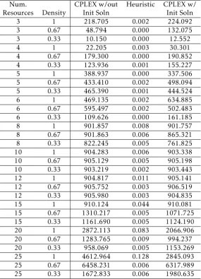
Table 7: Average runtime (in seconds) for each solution approach to find a solution. For those cases where CPLEX is not able to find a feasible solution within the time-limit, the returned time by CPLEX is still used in this computation.

Num. CPLEX w/out Heuristic CPLEX w/

Resources Density Init Soln Init Soln

3 1 218.705 0.002 224.092

3 0.67 48.794 0.000 132.075

3 0.33 10.150 0.000 12.552

4 1 22.205 0.003 30.301

4 0.67 179.300 0.000 190.852

4 0.33 123.936 0.001 155.227

5 1 388.937 0.000 337.506

5 0.67 433.410 0.002 498.094

5 0.33 465.390 0.001 444.524

6 1 469.135 0.002 634.885

6 0.67 595.497 0.002 502.483

6 0.33 109.626 0.000 161.185

8 1 901.857 0.008 901.757

8 0.67 901.863 0.006 865.321

8 0.33 822.245 0.005 761.825

10 1 904.283 0.006 903.338

10 0.67 905.129 0.005 905.198

10 0.33 903.219 0.002 903.443

12 1 904.817 0.011 905.141

12 0.67 905.752 0.003 906.519

12 0.33 905.980 0.003 904.835

15 1 910.124 0.044 910.081

15 0.67 1310.217 0.005 1071.725

15 0.33 1161.690 0.005 1124.190

20 1 2872.113 0.083 2066.906

20 0.67 1283.765 0.009 994.237

20 0.33 958.069 0.005 1153.269

25 1 4612.964 0.128 2845.093

25 0.67 6458.231 0.006 6317.989

25 0.33 1672.833 0.006 1980.635

is also able to find a better solution on average than is the heuristic. However, after this point, for almost all cases the heuristic is finding a better solution than is CPLEX without an initial solution. Again, this is to be expected, because as the size of the problem grows, commercial software will have more difficulty in solv-ing the larger problems and the heuristic will begin to find better solutions. But in comparing the heuristic with CPLEX with an initial solution, the average nor-malized distance between solutions is never that large on average, showing that the heuristic is able to find a good-quality solution as compared with commercial software.

fxh_j, sh_j−_fxc

j, scj

fxc_j, sc_j (35)

Table 6 presents, for those IGRs chosen to be routed, the mean time delay between IGR generation and IGR consumption. Column 3 of Table 6 shows the mean delay for the CPLEX solution when no initial solution is provided, Column 4 shows the mean delay for the

heuristic solution, while Column 5 shows the mean delay for the CPLEX solution when an initial solu-tion is provided. As is clear from this table, for those IGRs routed, the heuristic is able to route them much quicker than is CPLEX. This is regardless of the size of the problem. The rationale for this is that the heuristic is choosing IGRs to route in a greedy way, while CPLEX considers the routing of all IGRs simultanously.

longer to complete. This is due to CPLEX not being able to ‘halt’ processing exactly when the time limit is reached.

5

Conclusions

and

Future

Re-search

In this research, we have examined the problem of rout-ing information amongst a set of resources, when there exists a dynamic communication network topology with limited, time-varying, bandwidth, over a given time horizon. A rigorous mathematical formulation was developed to model the problem, with the objec-tive being to minimize the time delay of the informa-tion that can be routed while at the same time max-imizing the size of the information routed. This for-mulation is nonlinear, but a linearized version can be derived through standard techniques of operations re-search. As the problem is NP-hard, a heuristic has been developed to efficiently find good-quality solutions. Numerous Monte-Carlo simulations were performed on problems with varied resources and communica-tion network topology density. As can be seen in the results, for smaller sized problems commercial soft-ware is able to find a better solution on average than is the heuristic. And when the commercial software uses as input the solution found by the heuristic, even better results are obtained. As the size of the prob-lem increases, however, the heuristic begins finding much better solutions compared with the commercial software. And even when the commercial software is provided the heuristic solution as input, the commer-cial software is not able to improves significantly on this solution. Looking at the metric of the actual time-delay for those IGRs chosen to be routed, it is clear that the heuristic is better able to route those chosen IGRs. When coupled with the time needed for the heuristic to find a good quality solution versus the commercial software, it is clear that the heuristic is outperforming the commercial software.

Future research includes looking at specific net-work topology structures from realistic military and civil applications, considering the related problem of finding the minimum network temporal connectivity necessary to ensure certain information is able to be routed within time bounds, as well as considering the problem from a decentralized control paradigm, when no resource has knowledge about the network as a whole, but rather must consider only local network knowledge and make independent routing decision. In addition, incorporating the concept of network packet errors will provide added complexity and realism to the problem and scenarios considered.

Conflict of Interest The authors declare no conflict of interest.

Acknowledgment This research was Supported by Office of Naval Research Project N00014-15-C-5163.

References

[1] M. J. Hirsch, A. Sadeghnejad, and H. Ortiz-Pena, “Shortest paths for routing information over temporally dynamic com-munication networks,” inProceedings of the IEEE Military Communications Conference, pp. 587–591, 2017.

[2] I. Akyildiz, W. Su, Y. Sankarasubramaniam, and E. Cayirci, “Wireless sensor networks: A survey,”Computer Networks, vol. 38, pp. 393–422, 2002.

[3] J. Al-Karaki, , and A. Kamal, “Efficient virtual-backbone rout-ing in mobile ad hoc networks,” inElsevier Computer Networks, vol. 52, pp. 327–350, 2008.

[4] E. Huang, W. Hu, J. Crowcroft, and I. Wassell, “Towards com-mercial mobile ad hoc network applications: a radio dispatch system,”6th ACM International Symposium on Mobile Ad Hoc Networking and Computing, pp. 355–365, 2005.

[5] “Army 18.1 Small Business Innovation Research (SBIR) Pro-posal Topic 025: An Adaptively Covert, High Capacity RF Communications / Control Link,” tech. rep., 2018.

[6] “Air Force 18.1 Small Business Innovation Research (SBIR) Proposal Topic 019: Novel Battle Damage Assessment Using Snesor Networks,” tech. rep., 2018.

[7] C. Howard, “UAV command, control, and communication,” Military and Aerospace Electronics, vol. 24, 2013.

[8] B. Vignac, F. Vanderbeck, and B. Jaumard, “Reformulation and decomposition approached for traffic routing in optical networks,”Networks, vol. 67, pp. 277–298, 2016.

[9] J. Brodkin, “Tropical storm Harvey takes out 911 centers, cell towers, and cable networks,”ars Technica, August 28 2017.

[10] L. K. Comfort and T. W. Haase, “Communication, choerence, and collective action: The impage of Hurrican Katrina on the communication infrastructure,”Public Works Management & Policy, vol. 11, no. 1, pp. 1–16, 2006.

[11] U.S. Air Force, “USAF Strategic Master Plan,” tech. rep., 2015.

[12] “Air Force 17.1 Small Business Innovation Research (SBIR) Proposal Topic 047: Resilient Communication for Contested Autonomous Manned/Unmanned Teaming,” tech. rep., 2017.

[13] D. L. Hall and J. Llinas, “An introduction to multisensor data fusion,” inProceedings of the IEEE, vol. 85-1, pp. 6–23, 1997.

[14] E. Bosse, J. Roy, and S. Wark, eds.,Concepts, Models, and Tools for Information Fusion. Artech House, 2007.

[15] F. A. A. U.S. Department of Transportation, “Aviation Main-tenance Technician Handbook – Airframe, Volume 2,” tech. rep., 2012.

[16] “Navy 17.A Small Business Technology Transfer (STTR) Pro-posal Topic T029: Multi-Vehicle Collaboration with Minimal Communication and Minimal Energy,” tech. rep., 2017.

[17] I. Jebadurai, E. Rajsingh, and G. Paulraj, “Enhanced dynamic source routing protocol for detection and prevention of sink-hole attack in mobile ad hoc networks,”International Journal of Network Science, vol. 1, pp. 63–79, 2016.

[18] U. Paul, M. Buddhikot, and S. Das, “Opportunistic traffic scheduling in cellular data networks,”IEEE International Sym-posium on Dynamic Spectrum Access Networks, pp. 339–349, 2012.

[19] J. Al-Karaki, R. Ul-Mustafa, and A. Kamal, “Data aggrega-tion and routing in wireless sensor networks: Optimal and heuristic algorithms,” inElsevier Computer Networks, vol. 53, pp. 945–960, 2009.

[21] M. J. Hirsch and H. Ortiz-Pena, “Information supply chain optimization with bandwidth limitations,”International Trans-actions in Operational Research, vol. 24, no. 5, pp. 993–1022, 2017.

[22] E. Grotli and T. Johansen, “Path and data transmission plan-ning for cooperating uavs in delay tolerant network,” in Globe-com Workshop, pp. 1568–1573, IEEE, 2012.

[23] S. Basagni, C. Petrioli, R. Petroccia, and M. Stojanovic, “Opti-mizing network performance through packet fragmentation in multi-hop underwater communications,” inOCEANS, pp. 1–7, IEEE, 2010.

[24] P. Kansal and A. Bose, “Bandwidth and latency requirements for smart transmission grid applications,”IEEE Transactions on Smart Grid, vol. 3, pp. 1344–1352, 2012.

[25] M. Greenberg,Advanced Engineering Mathematics. Pearson, 2nd ed., 1998.

[26] L. Wolsey,Integer Programming. Wiley, 1998.

[27] I. CPLEX, “http://www-01.ibm.com/software/commerce /optimization/cplex-optimizer/,” Accessed January 2017.

[28] LINDO, “http://www.lindo.com/,” Accessed July 2016.

[29] J. Lenstra and A. R. Kan, “Complexity of vehicle and schedul-ing problems,”Networks, vol. 11, pp. 221–227, 1981.

[30] M. Solomon and J. Desrosiers, “Time window constrained rout-ing and schedulrout-ing problem,”Transportation Science, vol. 22, pp. 1–13, 1988.

[31] M. Dror and P. Trudeau, “Split delivery routing,”Naval Re-search Logistics, vol. 37, pp. 383–402, 1990.

[32] G. Ausiello, M. Protasi, A. Marchetti-Spaccamela, G. Gam-bosi, P. Crescenzi, and V. Kann,Complexity and Approximation: Combinatorial Optimization Problems and Their Approximability Properties. Springer-Verlag New York, Inc., 1st ed., 1999.

[33] M. R. Garey and D. S. Johnson,Computers and Intractability: A Guide to the Theory of NP-Completeness. New York, NY, USA: W. H. Freeman & Co., 1979.

[34] Matlab, “http://www.mathworks.com/products/matlab/,” Accessed January 2017.

[35] B. Szymanski, X. Lin, A. Asztalos, and S. Sreenivasan, “Failure dynamics of the global risk network,”Scientific Reports, vol. 5, pp. 1–14, 2015.

[36] R. Liu, M. Li, and C. Jia, “Cascading failures in coupled works: The critical role of node-coupling strength across net-works,”Scientific Reports, vol. 6, pp. 1–6, 2016.