A. Heibig, F. Filbet, L. I. Palade, Editors
APPROXIMATING THE TRACE OF ITERATIVE SOLUTIONS AT THE
INTERFACES WITH NONUNIFORM FOURIER TRANSFORM AND SINGULAR
VALUE DECOMPOSITION FOR COST-EFFECTIVELY ACCELERATING THE
CONVERGENCE OF SCHWARZ DOMAIN DECOMPOSITION
Damien Tromeur-Dervout
1R´esum´e. Cet acte traite de la repr´esentation des solutions it´er´ees aux interfaces de la m´ethode de d´ecomposition de domaine de type Schwarz afin d’approximer de mani`ere adaptative son op´erateur d’er-reur aux interfaces des sous domaines. Ceci permet de construire de mani`ere ´economique l’acc´el´eration de la convergence de la m´ethode it´erative en ´etendant la technique d’acc´el´eration de la convergence de Aitken au cas vectoriel. La premi`ere repr´esentation est fond´ee sur la construction d’une transform´ee de Fourier discr`ete non uniforme d´efinie sur un maillage non r´egulier. Nous montrons comment construire une base de Fourier de dimension N+1 sur ce maillage `a partir de la construction num´erique d’une forme sesquilin´eaire, son exactitude pour les polynˆomes trigonom´etriques de degr´e N/2, et num´eriquement sa capacit´e d’approximation spectrale d´ependante de la continuit´e de la fonction `a approximer. La d´ecroissance des modes de Fourier de la trace de la solution it´er´ee aux interfaces nous fournis une esti-mation pour s´electionner de mani`ere adaptive les modes intervenant dans l’acc´el´eration. Le d´efaut de cette approche est d’ˆetre d´ependant de la continuit´e de la solution it´er´ee aux interfaces. La deuxi`eme repr´esentation, purement alg´ebrique, utilise une d´ecomposition en valeurs singuli`eres des solutions it´er´ees aux interfaces pour fournir un ensemble de vecteurs singuliers orthogonaux dont les valeurs sin-guli`eres associ´ees fournissent une estimation pour adapter l’acc´el´eration. La m´ethode Aitken-Schwarz r´esultante est ensuite appliqu´ee au calcul `a grande ´echelle pour r´esoudre un ´ecoulement 3D en milieu poreux mod´elis´e par l’´equation de Darcy lin´eaire o`u la perm´eabilit´e suit une distribution al´eatoire log-normale.
1 University of Lyon, University Lyon1 CNRS Institut Camille Jordan UMR5208,
43 Bd du 11 Novembre 1918, F-69150 Villeurbanne cedex, France
c
EDP Sciences, SMAI 2013
Abstract. This paper deals with the representation of the trace of iterative Schwarz solutions at the interfaces of domain decomposition to approximate adaptively the interface error operator. This allows to build a cost-effectively accelerating of the convergence of the iterative method by extending to the vectorial case the Aitken’s accelerating convergence technique. The first representation is based on the building of a nonuniform discrete Fourier transform defined on a non-regular grid. We show how to construct a Fourier basis of dimension N+1 on this grid by building numerically a sesquilinear form, its exact accuracy to represent trigonometric polynomials of degree N / 2, and its spectral approximation property that depends on the continuity of the function to approximate. The decay of Fourier-like modes of the approximation of the trace of the iterative solution at the interfaces provides an estimate to adaptively select the modes involved in the acceleration. The drawback of this approach is to be dependent on the continuity of the trace of the iterated solution at the interfaces. The second representation, purely algebraic, uses a singular value decomposition of the trace of the iterative solution at the interfaces to provide a set of orthogonal singular vectors of which the associated singular values provide an estimate to adapt the acceleration. The resulting Aitken-Schwarz methodology is then applied to large scale computing on 3D linear Darcy flow where the permeability follows a log normal random distribution.
Introduction
The Schwarz domain decomposition (DD) method[35] is a very attractive numerical method for the parallel computing as it needs only to update the boundary conditions on the artificial interfaces generated by DD. Thus only local communications between the neighboring sub-domains are needed. Nevertheless, the main drawback of this method is its slow rate of convergence which depends on the partial differential problem, the geometry of the sub-domains, and the size of the overlap when overlap is present. The idea of using Aitken acceleration [20] on the classical additive Schwarz DD method was introduced in [18]. These authors have called the corresponding method the Aitken-Schwarz (AS) method. They have shown its great numerical performances on linear and nonlinear elliptic problems discretized by a five-point scheme on a rectangular Cartesian grid [2]. It was shown that this technique gives efficient metacomputing time to solve elliptic linear separable problem with the Laplacian operator and nonlinear problem such as the Bratu problem [5] in three dimensional space with a broad network of supercomputers linked by a regular internet connection.
basis and decay in the coefficients of the approximation that provide an estimate to adapt the vectorial Aitken acceleration technique of the Schwarz DD.
The plan of the paper is the following. In section 1 we present the Schwarz DD method and its convergence property when applied to linear elliptic problems. Then section 2 focuses on the Aitken’s acceleration of the convergence of Schwarz DD method for linear separable operators on regular meshes. Difficulties arise when linear non separable operators and/or with non regular mesh on the interfaces are under consideration. Section 3 defines the nonuniform Fourier-like transforms and the corresponding approximation of the error operator on the interface [14]. Section 4 extends the methodology with an Aitken acceleration based on the singular value decomposition of the solution at the artificial boundaries. Then this method becomes totally mesh free [39]. Moreover, the decreasing of the singular values gives an a priori criterion to select the singular vectors involved in the Aitken’s acceleration operator approximation. This allows solving the large 3D computation of the linear Darcy equation where the permeability field follows a random log normal distribution law [3] in section 5.
1.
The Schwarz domain decomposition method and its properties
In the Schwarz DD method the problem is reduced to solve a problem on the interface. The trace theorem (see for example [[37],p.9] and references) allows to define a restriction of the solution on the interface and also to extend the interface solution in the whole subdomains. Let Ω ⊂Rn be a bounded domain with Lipschitz
boundary Γ := ∂Ω. For any u belonging to the Hilbert space H1(Ω) there exists the trace γ
0u ∈ H1/2(Γ)
satisfying
||γ0u||H1/2(Γ) ≤ cT.||u||H1(Ω). (1)
Vice-versa, for anyu∈H1/2(Γ) there exists a bounded extensionεu
∈H1(Ω) satisfyingγ
0εu=uand
||εu||H1(Ω) ≤ cIT.||u||H1/2(Γ). (2)
Consider a scalar second order uniformly elliptic boundary value problem with Dirichlet boundary condition (BC):
L(x)u(x) = f(x), forx∈Ω, γ0u(x) = g(x), forx∈Γ,
(3)
where the partial differential operatorL(x), x∈Ω is given by
L(x)u(x) = −Σni,j=1 ∂
∂xj[aji(x) ∂
∂xiu(x)] (4)
with aji =aij ∈ L∞(Ω), i, j = 1, . . . , n. L(.) is assumed to be uniformly elliptic, i.e. there exists a positive
constantc0 independent ofx∈Ω such that for allx∈Ω
Σni,j=1aji(x)ξjξl≥c0.|ξ|2,∀ξ∈Rn (5)
We assume f ∈H−1(Ω),g
∈H1/2(Γ).
The conormal derivative operatorγ1 is given by
γ1u(x) := Σni,j=1nj(x)[aji(x)
∂
∂xiu(x)], ∀x∈Γ (6)
Foru, v∈H1(Ω), we define the symmetric bilinear form
a(u, v) := Σni,j=1
Z
Ω
∂
∂xjv(x)aji(x) ∂
∂xiu(x)dx (7)
which is bounded inH1(Ω)
|a(u, v)| = c.||u||H1(Ω)||v||H1(Ω),∀u, v∈H1(Ω). (8)
Using the Green’s second formula foru, v∈H1(Ω),
a(u, v) = Z
Ω
L(x)u(x)v(x)dx+ Z
Γ
γ1u(x)γ0v(x)dsx (9)
LetH1 0(Ω) :=
v∈H1(Ω) :γ
0v(x) = 0,forx∈Γ . Using (9), the variational formulation of Eq (3) is :
Findu∈H1(Ω) satisfyingγ
0u(x) =g(x),∀x∈Γ such that
a(u, v) = Z
Ω
f(x)v(x)dx,∀v∈H1
0(Ω) (10)
From the uniform ellipticity (5) and Poincar´e inequality, we get that the bilinear form a(., .) is elliptic on
H1
0(Ω). Using Eq (8),Eq (5) , and the generalized Lax-Milgram lemma due to Necas [28], we conclude that
problem (3) has a unique solution u∈H1(Ω).
1.1.
The Dirichlet-Neumann Map
The Dirichlet-Neuman map connects the solution and its normal derivative at the domain boundary. The DD method can be formulated in terms of this Dirichlet to Neumann map. The unique solution of problem (3)
u∈H1(Ω) can be written as u=u
0+εg, where u0 corresponds to the solution of Eq (3) with homogeneous
Dirichlet BC andεg satisfies the homogenous Eq (3) with non-homogeneous Dirichlet BC . We define a linear functional
l(w) := a(u, εw)− Z
Ω
f(x)εw(x)dx, forw∈H1/2(Γ). (11)
Applying the Riez representation theorem, there exists aλ∈H−1/2(Γ) such that
hλ, wiL2(Γ) = l(w), ∀w∈H
1/2(Γ). (12)
Hence,λ∈H−1/2(Γ) is the conormal derivativeγ
1u, as it satisfies:
Z
Γ
λ(x)w(x)dsx = a(u0+εg, εw)−
Z
Ω
f(x)εw(x)dx, for allw∈H1/2(Γ). (13)
We then have defined a map from the given data (f, g) to the associated Neumann boundary data λ:=γ1u.
In particular, for a fixedf and varying Dirichlet boundary datag=γ0u, we have defined a Dirichlet-Neumann
map which may be written as
γ1u(x) = Sg(x)−N f(x),∀x∈Γ (14)
1.2.
The Generalized Schwarz Alternating Method
Let us first recall the Generalized Schwarz Alternating Method (GSAM) introduced by [12] that gathers several Schwarz techniques [32]. For the sake of simplicity, let us consider the case where the whole domain Ω is decomposed into two sub-domains Ω1 and Ω2, with overlapping or not, defining two artificial boundaries
Γ1, Γ2. Let us define ¯i = mod(i,2) + 1 and Ω11 = Ω1\Ω2, Ω22 = Ω2\Ω1, Ω12 = Ω1∩Ω2, Ω11 = Ω1\Ω12,
Ω22 = Ω2\Ω12 if there is an overlap. Let L(x) be the continuous elliptic operator. The GSAM solves until
convergence the problem (3) restricted to the domain Ω1 (respectively Ω2) with the Dirichlet B.C on∂Ω1 Γ1
(respectively∂Ω2Γ2) and a generalized BC: Λ1u1+λ1
∂u1
n1
=µ2on Γ1(respectively Λ2u2+λ2
∂u2
n2
=µ1), where
Λi are some operators andλi are constants. The valueµ2= Λ1u2+λ1
∂u2
∂n1
(respectivelyµ1= Λ2u1+λ2
∂u1
∂n2
)
is defined with respect to the solution u2 in Ω2 (respectively u1 in Ω1). As the solution on sub-domains Ωi
are unknowns, we iterate the solving, taking the generalized BC value µi with the solution obtained at the previous iterate in Ωi. The additive version of the GSAM consists to solve both sub-domains problems at the
same iterate while the multiplicative version the sub-domains problems are solved successively as updating the
µi values. Then GSAM can be summarized in Algorithm 1 that follows:
Algorithm 1GSAM: Multiplicative (M1=N2= 2n+ 1, M2= 2n+ 2, N1= 2n), Additive (M1=M2=n+ 1
N1=N2=n)
1: DO until convergence
2: Solve
L(x)uM1
1 (x) = f(x), ∀x∈Ω1, (15)
uM1
1 (x) = g(x), ∀x∈∂Ω1\Γ1, (16)
Λ1uM11 + λ1
∂uM1 1 (x)
∂n1
= Λ1uN21+λ1
∂uN1 2 (x)
∂n1
, ∀x∈Γ1 (17)
3: Solve
L(x)uM2
2 (x) = f(x), ∀x∈Ω2, (18)
uM2
2 (x) = g(x), ∀x∈∂Ω2\Γ2, (19)
Λ2uM22 + λ2
∂uM2 2 (x)
∂n2
= Λ2uN12+λ2
∂uN2 1 (x)
∂n2
, ∀x∈Γ2. (20)
4: Enddo
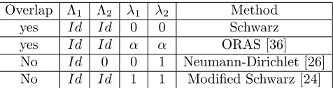
According to the specific choice of the operators Λi and the values of scalars λi, we obtain in Table 1 the
family of Schwarz DD techniques. If Λ1= Λ2=Idandλ1=λ2= 0 then the above multiplicative version is the
classical Multiplicative Schwarz. If Λ1= Λ2=constant >0 and λ1 =λ2= 1 then it is the modified Schwarz
Overlap Λ1 Λ2 λ1 λ2 Method
yes Id Id 0 0 Schwarz yes Id Id α α ORAS [36] No Id 0 0 1 Neumann-Dirichlet [26] No Id Id 1 1 Modified Schwarz [24]
Table 1. Derived methods obtained from the specific choices of the operators Λi and the
values of scalarsλi in the GSAM.
1.3.
Convergence property of the GSAM
Engquist & Zhao [12] showed that with an appropriate choice of the operators Λi this DD method converges
in two iterations. They established the proposition that follows:
Proposition 1.1. IfΛ1(or Λ2) is the Dirichlet to Neumann operator at the artificial boundaryΓ1 (orΓ2) for the corresponding homogeneous PDE in Ω2 (orΩ1) with homogeneous BC on∂Ω2∩∂Ω(or∂Ω1∩∂Ω) then the Generalized Schwarz Alternating method converges in two steps.
The GSAM method converges in two steps if the Dirichlet-Neumann operators Λi, i = 1,2, are available.
These operators are not local to a sub-domain but they link up together all the sub-domains if their number is greater than two.
In the Aitken-Schwarz methodology introduced by [17, 18], only the purely linear convergence property of the Schwarz method (for local linear operator in subdomain) is used. Consequently, no direct approximation of the Dirichlet-Neumann map is used, but an approximation of the operator of error linked to this Dirichlet-Neumann map is performed.
The pure linear convergence of the GSAM can be established as follows. Define the projection operator
Pi : H1(Ω
i)→H1(Ωii) to be the restriction from Ωi to Ωii. Denote Si (respectively Sii) to be the Dirichlet
to Neumann map operator in Ωi (respectively Ωii) on Γi (respectively Γ¯i). LetRi be the restriction operator
from H1(Ω
i) to H1/2(Γi) andR∗i be the right inverse operator ofRi, i.e,RiR∗i =I,∀g∈H
1/2(Γ
i), L(x)R∗ig=
0, R∗
ig=g onΓi, R∗ig= 0on ∂Ωi\Γi. Let Rii be the corresponding operator in Ωii,∀g ∈H1/2(Γ¯i), L(x)R∗iig=
0, R∗
iig=g onΓ¯i, Rii∗g= 0on ∂Ωii\Γ¯i
The following proposition (see [[12],p.354]) establishes the convergence of the GSAM.
Proposition 1.2. After one cycle of iteration on the error functionen
i =u−u n
i inΩi for the GSAM, we have for{i, j}={1,2}, i6=j:
en
i = R∗i(Λi+λiSi)−1(Λi−λiSjj)RjjPjR∗j(Λj+λjSj)−1(Λj−λiSii)RiiPi(eni−2). (21)
For the non-overlapping Schwarz (Γ1= Γ2, Pi=Id,Rii=Ri), Eq (21) is reduced to
en
i = R
∗
i(Λi+λiSi)−1(Λi−λiSj)(Λj+λjSj)−1(Λj−λjSi)Rieni−1. (22)
Consequently, by applyingRi to Eq (22) we see that the trace of the error on Γi satisfies:
Rien
i = RiR
∗
i | {z }
Id
(Λi+λiSi)−1(Λi−λiSj)(Λj+λjSj)−1(Λj−λjSi)
| {z }
P
Rieni−1.
The trace of the error converges purely linearly as the error operatorPdoes not depend of the Schwarz iteration. The Aitken-Schwarz methodology uses this property to accelerate the convergence of the Schwarz algorithm to the right solution at the artificial interface.
Remarque 1.3. The same convergence applies in the general case of GSAM with applying the operatorRiiPi
1.4.
Connexion between Steklov-Poincar´
e and Schur complement operators
For simplicity, let us consider two subdomains with no overlap. Then the discretization of Eq (3), with either finite volume or second order finite differences, leads to the following matrix system:
Au =
A11 0 A13
0 A22 A23
A31 A32 A (1) 33 +A
(2) 33 u1 u2 u3 = f1 f2
f3(1)+f (2) 3
(23)
whereu1 andu2 denote the vector of interior unknowns in sudomains Ω1 and Ω2, respectively, andu3 denotes
the vector of remaining nodal unknowns on Γ. The interior nodal unknowns can be formally eliminated from Eq (23) by writting:
u1=A−111(f1−A13u3),
u2=A−221(f2−A23u3),
(24)
and by denoting
S1=A (1)
33 −A31A−111A13, g1=f (1)
3 −A31A−111f1,
S2=A (2)
33 −A32A−221A23, g2=f (2)
3 −A32A−221f2,
(25)
we obtain the interface Schur complement system
Su3= (S1+S2)u3=g1+g2=g (26)
Note that the following identity holds (see [27]):
ˆ
A11
0
S1x3
=
A
11 A13
A31 A (1) 33
−1 0
S1u3
=
A11 A13
0 I −1 0 u3 (27)
The matrix ˆA11 corresponds to the discrete stiffness matrix on subdomain Ω1with homogeneous Dirichlet BC
on the external boundary segment and Neumann BC on the interface boundary Γ. So that, the matrix vector product S1x3 is simply the discrete conormal derivative on Γ associated with the homogeneous equivalent of
Eq(14) on the sub-domain Ω1 with zeros boundary data on∂Ω1\Γ and prescribed non zeros valuesu3 on Γ (i.e
for S2u3). These matrix vector products are the discrete equivalents of the Steklov-Poincar´e operator on the
respective subdomains.
At the discrete level the pure linear convergence of the GSAM holds, and the operator errorP on trace error involves the local Schur complement of al the subdomains. In practice, some algebraic approximations of these local Schur complements are used (see [8, 15, 19]), while in the Aitken-Schwarz methodology, we do not search to approximate the local Schur complement but to build the discrete matrix P or an approximation of this matrixP, in order to accelerate the convergence.
2.
Aitken-Schwarz Method for Linear Operators
2.1.
Aitken-Schwarz 1D problem case
In the case of the additive GSAM (Λ1 = Λ2 = Id, λ1 = λ2 = 0) with two overlapping subdomains, the
iterations of the errors at the interfaces can be written as follows:
en+1
1 (Γ2)
en2+1(Γ1)
=
0 δ2
δ1 0
en
1(Γ2)
en
2(Γ1)
(28)
Consequently, ifδ1, δ2 are not known, they can be deduced from the relation:
en1+2(Γ2) en1+1(Γ2)
en+2
2 (Γ1) en2+1(Γ1)
en1+1(Γ2) en1(Γ2)
en+1
2 (Γ1) en2(Γ1)
−1 =
0 δ2
δ1 0
=P (29)
Ifδ1δ26= 1, the Aitken acceleration gives the exact solution at the interfaces :
u∞(Γ1) = [−u12+δ2u01+δ2(δ1u02−u 1
1)]/(δ1δ2−1), (30)
u∞(Γ2) = [−u11+δ1u02+δ1(δ2u01−u 1
2)]/(δ1δ2−1) (31)
An additional solve of each of the subproblems with BCs u∞
Γi gives the solution. The Aitken acceleration
thus transforms the additive Schwarz procedure into an exact solver regardless of the speed of convergence of the original Schwarz method. We observe thatδ1, δ2 are dependent only on the operator and the partitioning
of the domain. δi, i={1,2} for example can be computed before hand as follows. Letvi be the solution of
L(x)vi(x) = 0, ∀x ∈ Ωi, withvi|Γi = 1. (32)
We have then δ¯i=vi|Γ¯i. vi can be computed numerically and possibly analytically if the differential operator L(x) is simple enough. Whenδi, i={1,2}is known, we need only one Schwarz iterate to accelerate the interface and an additional solve for each subproblem. This is a total of two solves per sub-domain.
2.2.
The Aitken-Schwarz method on linear separable operators and regular mesh on
ar-tificial interface
In order to show the case with several subdomains, consider the 3D Poisson equation, where the domain is discretized with regular size steps in each direction, and the separable Poisson operator is approximated using second order finite differences. We used additive Schwarz with Dirichlet BC (Λi =Idand λi = 0 in GSAM).
The overlap is set to the minimum of one cell or one step size as the Aitken-Schwarz method is not related to the rate of convergence but only to the pure linear convergence or divergence property. As we use a regular mesh at the artificial interfaces, we can proceed as previously with writing the solution on the artificial interfaces generated by the Schwarz algorithm in a sine expansion in they andz directions. Thus for:
−( ∂
2
∂x2 +
∂2
∂y2 +
∂2
∂z2)u(x, y, z) =f(x, y, z),∀(x, y, z)∈Ω = [0, π] 3,
u(x, y, z) = 0,∀(x, y, z)∈∂Ω.
(33)
we search foru(x, y, z) =P
1≤j≤ny
P
1≤k≤nzujkˆ (x) sin(jy) sin(kz). The 3D problem is equivalent to the
follow-ingny×nz discrete problems:
−ujk,iˆ +1+ 2ˆujk,i−ujk,iˆ −1
h2
x
+λjujk,iˆ +λkujk,iˆ = ˆfjk,i,1≤i≤Nx−1
ˆ
ujk,0=αjk
ˆ
ujk,nx =βjk
where λj = h42 y sin
2
(jhy
2 ) (respectively λk = 4
h2 z sin
2
(khz
2 )) are the eigenvalues of the
∂2
∂y2 (respectively ∂2 ∂z2)
operator with homogeneous BC approximated by a second order finite differences scheme with a regular step sizehy (respectively hz). hx represents the regular step size in thexdirection.
The domain in the x direction is split in q subdomains Ωi = (Xil, Xir), i = 1..q with X2l < X1r < X3l <
Xr
2, ..., Xql < Xqr−1. For the sake of simplicity we choose the subdomains Ωi to have the same size, discretized
with a regular step size hx = Xil−X r i
nx given nx+ 1 points xl =X l
i +l hx. Then the discrete error ˆei of the
Schwarz algorithm on subdomain Ωi for the modejk at iteraten+ 1 satisfies :
ˆ
eni+1(xl+1)−(2 +λjhx+λkhx)ˆeni+1(xl) + ˆe n+1
i,l−1(xl−1) = 0, 1≤l≤nx−1,
ˆ
eni+1(X l
i) = ˆeni−1(Xil),
ˆ
en+1
i (Xir) = ˆeni+1(Xir).
(35)
The generic solution of this system of linear equations writes:
ˆ
en+1
i (xl) =C1Z1l+C2Z2l,0≤l≤nx (36)
whereZ1 andZ2 are the roots of−Z2+ (2 +λjhx2+λkh2x)Z−1 = 0. The two constant parametersC1andC2
are given by the BCs:
1 1
Znx
1 Z nx 2 C1 C2 = ˆ en i−1(Xil)
ˆ
en i+1(Xir)
(37)
Thus the error on domains Ωi−1 and Ωi+1 at iteraten+ 1 depends on the error at iterate non domain Ωi.
One can write:
ˆ
eni−+11(X
r i−1)
ˆ
en+1
i+1(Xil+1)
=
δil,l δ l,r i δir,l δir,r
ˆ
en i(Xil)
ˆ
en i(Xir)
(38)
Then coefficientδil,l(respectivelyδ r,l
i ) is the value of ˆeni(Xir−1) (respectively (ˆeni(Xil+1)) when the BCs on domain
Ωi are ˆeni(Xil) = 1 and ˆeni(Xir) = 0 while coefficientδ l,r
i (respectivelyδ r,r
i ) is the value ˆeni(Xir−1) (respectively
ˆ
en
i(Xil+1)) when the BCs on domain Ωi are ˆeni(Xil) = 0 and ˆe n+1
i (Xir) = 1. Consequently, these values can be
found analytically once for all by computing the valuesC1 andC2associated to the BCs and by evaluating the
function ˆen
i(x) inX r
i−1andX
l
i+1. If we choose a minimum overlap ofhxbetween subdomains (X
r i−1=X
l i+hx
andXl
i+1=Xir−hx) we obtain:
Pi def=
δil,l δ l,r i δir,l δ
r,r i =
Z1Z2(Z2nx−1−Z
nx−1
1 )
Znx 2 −Z
nx 1
(Z1Z2)nx−1(Z2−Z1)
Znx 2 −Z
nx 1
Z2−Z1
Znx 2 −Z
nx 1
Znx−1
2 −Z
nx−1 1
Znx 2 −Z
nx 1 (39)
The matrixPi can also be computed numerically from three iterations as
Pi =
ˆ
en+2
i−1(X
r i−1) eˆ
n+1
i−1(X
r i−1)
ˆ
en+2
i+1(Xil+1) ˆe
n+1
i+1(Xil+1)
ˆ
eni+1(X l
i) eˆni(Xil)
ˆ
en+1
i (Xir) eˆni(Xir) −1
(40)
whereeni+2=u n+2
i −u n+1
i
We noteel,ni =e n i(X
l i),e
r,n i =e
n i(X
r i) and ˜e
n thenthiterated error restricted at the interfaces, i.e
˜
en = (el,n
2 , e
r,n
1 , e
l,n
3 , e
r,n
2 , ..., e
l,n q , e
r,n q−1)
LetP be the matrix that links the error on artificial interfaces of the Schwarz DD.P has the following penta-diagonal structure:
0 δr
1 0 0 ....
δ2l,l 0 0 δ
l,r
2 ...
δr,l2 0 0 δ
r,r
2 ...
... δl,lq−1 0 0 δ
l,r q−1
... δr,lq−1 0 0 δ
r,r q−1
... 0 0 δr q 0
From the equality
˜
en+1=P(˜en),
one writes the Aitken acceleration as follows:
˜
u∞= (Id−P)−1(˜un+1
−Pu˜n). (42)
If the additive Schwarz method converges, then||P||<1 andId−P is non singular.
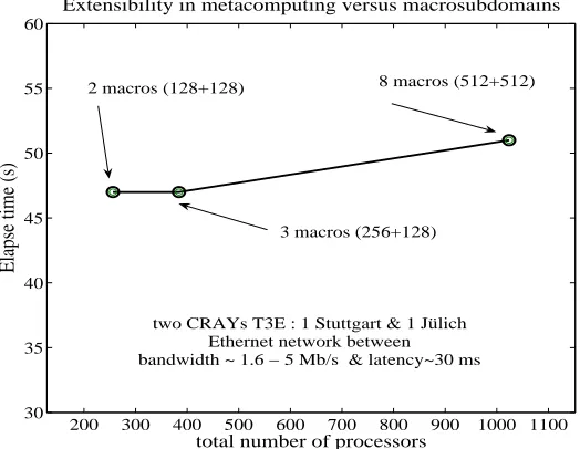
Let us report the results obtained to solve the Poisson equation on a metacomputing framework based on networks that provide as low a level of performance as Ethernet [2]. For large scale metacomputing experiments, we are using up to three Cray T3E located in Stuttgart, Pittsburgh, and J¨ulich with 512 processors cadenced to 450Mhz , 40Mhz and 375 Mhz, a latency of 12µsand a communication bandwidth of 320M B/s.
The main challenge is to combine the Aitken-Schwarz DD method with an efficient parallel subdomain solver as PDC3D in order to have a highly efficient solver for the 3D Poisson operator for metacomputing environments. PDC3D [34],[33], is a parallel fast direct solution method for linear systems with separable block tridiagonal matrices. The method under consideration has the arithmetical complexityO(Nlog2N), and is closely related to the cyclic reduction method. This very efficient solver requires a high performance communication network mainly due to the necessary global reduction operations, to gather the partial solution. It reaches a very good scalability for a CrayT3E.
For all our experiments, the bandwidth fluctuated in the range of 1.6 −5M b/s and the latency was about 30ms. We used the PACX-MPI communication library [7] that used the best communication network available for exchange of data between processors. The mpi vendor implementation is used when two nodes of a same machine must communicate and MPI with TCP-IP protocol is used in a user transparent way when two nodes of different machines have to communicate.
We have a three-dimensional DD and a two-level algorithm combining Aitken-Schwarz in thex-direction and PDC3D solver in theyandzdirections for subdomain problems local to machines (named macro) that matches the hierarchy of the network speed and access to memory speed in a distributed GRID environment. The number of grid points in Aitken DD directionxis balanced in such a way that PDC3D requires the same CPU time on each system. We defined the barrier between low and medium size frequencies in each space variable to be 1/4 of the number of waves. We did not accelerate the upper half of the frequencies. We checked that the impact on the numerical error against an exact polynomial solution is in the interval [10−7,10−6] for our test cases with
200 300 400 500 600 700 800 900 1000 1100 30
35 40 45 50 55 60
2 macros (128+128)
3 macros (256+128)
8 macros (512+512)
two CRAYs T3E : 1 Stuttgart & 1 Jülich Ethernet network between bandwidth ~ 1.6 − 5 Mb/s & latency~30 ms
total number of processors
Elapse time (s)
Extensibility in metacomputing versus macrosubdomains
Figure 1. Scalability of the Aitken Schwarz algorithm for the 3D Poisson problem in various
metacomputing environments with CrayN and CrayS.
2.3.
The Aitken-Schwarz method for linear non separable operators and/or non regular
mesh on artificial interface
For non-regular interface discretization the classical Fourier transform is not available. Some generalizations of the Fourier approach have been proposed in [16] and [1].
In [1] for a separable operator on a non regular mesh, an eigenvalue decomposition of the part of the operator acting in one direction is performed. Then the eigenvectors of this eigen-decomposition are used as generalized Fourier modes, the matrix P associated to each eigenvector being computed as in the regular mesh case by decomposing the solution trace on the interface in this eigenvector basis and then accelerating each generalized Fourier mode by Aitken’s formula before coming back in the ”physical” space to have the accelerated solution on the interface.
In [16], the eigen-pair is computed on the trace transfer operatorP which links the Schwarz iterate errors on the interface. Then three algorithms are proposed:
a a bandwidth approximation of matrixP: a block diagonal approximation of matrixP is performed and then the eigen-pair of this matrix block is searched,
b a coarse grid approximation of matrix P: it consists in defining a coarse grid and having restriction
Th/H and projectionTH/h to exchange between the fine grid and the coarse grid and then defining the coarse approximation of matrixP asTh/HP TH/h,
c a compact representation of the interface: a least square approximation of the Schwarz iterates solution is done on a regular mesh where a sine or cosine expansion is performed, depending on the BC.
Some accelerations have been obtained on finite volume with approach (b), better results come from (c) with very few modes in the expansion even if the convergence seems to retrieve the original rate of convergence after the first acceleration. Strategy (a) works quite well with a band approximation of matrixP of size 2Z+ 1 with
Z ={1,2,3}on a regular grid with a convection-diffusion operator closed to the Laplacian for which the matrix
to represent the property of pure linear of the sequence of iterate solution.
3.
Non Uniform Discrete Fourier Transform
We developed an original Non Uniform Discrete Fourier Transform (NUDFT) based on the values of the iterated solution at the interface mesh points. The most important feature of this approximation is that it provides a framework to perform adaptively the acceleration.
3.1.
Aitken-Schwarz in a multidimensional framework
Let us consider the multidimensional case with the discretized version of the problem (3). We restrict ourselves for simplicity to the two overlapping subdomains case and the multiplicative GSAM algorithm. In the multidimensional framework the main difficulty consists in defining a representation of the interface solutions that can produce a cheap approximation of the error transfer operator matrix P.
For a linear operator one can write the sequence of Schwarz iterates U0 Γ1
h, U 0 Γ2
h, U 1 Γ1
h, U 1 Γ2
h, ...
, then the error
between two Schwarz iterates behaves linearly. Errorsei
Γjh =U
i+1 Γjh −U
i
Γjh satisfy
eiΓ+11 h ei+1
Γ2 h
!
=P e i
Γ1 h ei
Γ2 h,
!
(43)
whereP represents the iteration error operator at artificial interfaces.
Let us consider now a discretisation of the interfaces with the meshes Γjh and let us denote Γh to be the
coarsest discretisation in the sense that it produces the smallest set of orthogonal vectors Φk that belong to Γh
with respect to a discrete Hermitian form [[., .]]. One can consider without loss of generality that these vectors satisfy [[Φk,Φk]] = 1,∀k∈ {0, ..., N}. Being given f ∈C∞(Γ) then one can define the vectorF(Γh) of discrete
values of a functionf on Γh. The set of vectors Φk defined on Γhshould also satisfy a density property in the
space ofC∞(Γ) functions whenN
→ ∞. I.e. ∀ >0,∃N ∈Nsuch that forn≥N the vectorFn=Pnk=0αkΦk
satisfies ||F(Γh)−Fn||∞< . Without this density property the acceleration of the convergence will converge
only to the part of the solution interface that can be approximated by the set of Φk. If the size of the set of
orthogonal vectors Φk is the size of the discrete interface then we have an exact (algebraic) approximation.
Consider the decomposition of the trace of the Schwarz solution in this orthogonal basisUΓ. LetUΓh be the
decomposition ofUΓ with respect to the orthogonal basis Φ.
UΓh = N X
k=0
αkΦk. (44)
Theαk represent the Fourier-like coefficients of the solution with respect to the basis Φ. The orthogonality of vectors Φk gives directly the value ofαk:
αk= [[UΓ,Φk]]. (45)
Let us consider now the decomposition of the traces in the basis Φ. Then the nature of the convergence does not change if we consider the error coefficients in the basis Φ instead of the error in the physical space. One can write an equivalent equation to Eq (43) but in the coefficient space. Letβi
Γjh be the coefficients of the error
ei
βi+1 Γ1
h βiΓ+12
h
!
=P[[.,.]]
βi
Γ1 h βi
Γ2 h
!
. (46)
This matrixP[[.,.]] has the same size as the matrix P. Nevertheless, we have more flexibility to define some
consistent approximation of this matrix, since we have access to a posteriori estimate based on the module value of the Fourier coefficients.
3.2.
Explicit building of
P
[[.,.]]The explicit building ofP[[.,.]]consists in computing how the basis functions Φk are modified by one Schwarz
iteration. Figure 2 describes the steps for constructing the matrix P[[.,.]]. Step (a) starts from the the basis
function Φk and gets its value on the interface in the physical space. Then step (b) performs two Schwarz
iterates with zero local right hand sides and homogeneous BCs on∂Ω =∂(Ω1∩Ω2). Step (c) decomposes the
trace solution on the interface in the basis Φ. Thus we obtain the columnkof the matrix P[[.,.]].
Figure 2. Steps to build theP[[.,.]] matrix
The full computation of P[[.,.]] can be done in parallel, but it needs as much local subdomain solves as
the number of interface points (i.e the size of the matrix P[[.,.]]). Its adaptive computation is required to
save computing time. The Fourier mode convergence gives a tool to select the Fourier modes that slow the convergence and have to be accelerated, contrary to the approach of [16], which builds an approximation of the operator in the physical space relatively to the trace solution on a coarse grid and then compute the Schur eigenvalue decomposition of this approximation. The adaptive Aitken-Schwarz algorithm can be described as follows:
Algorithm 2Adaptative Aitken-Schwarz
1: Perform two GSAM iterates.
1: Write the difference between two successive iterates in the Φ basis and select the component modes higher than a fixed tolerance and with the worst convergence slope. Set Index the array of selected modes.
1: Take the subset ˜v ofmFourier modes from 1 to max(Index).
2: Compute them×m P∗
[[.,.]] matrix associated to themmodes selected which is an approximation ofP[[.,.]]. 3: Accelerate themmodes with the Aitken formula:
˜
v∞= (Id−P[[∗.,.]])
−1(˜vn+1
−P[[∗.,.]]˜v
n). (47)
The arithmetical computing cost is greatly reduced ifmN. It is possible to optimize the implementation by computing a number of columns of matrix ˜P[[.,.]]during the Schwarz iteration on the problem. This considers
a new local problem with several right hand sides (one of them corresponds to the initial problem, the others are associated to local problems to compute the columns of ˜P[[.,.]] ). The constraint is to obtain a resulting
local problem that fits in the memory cache capacity. This can occur if there is a fast decay property of the components with the increase of the mode value as in the Fourier representation case. This paper will not focus on this aspect of the implementation because it depends on the hardware and on the considered problem.
3.3.
Fourier basis orthogonal with respect to a numerical Hermitian form
For nonregular meshes, the conjugate property of the standard Fourier basis (see [4]) is lost. First, we gave a new definition of the Fourier basis in order to keep the conjugate property with respect to the nonregular mesh points:
D´efinition 3.1. Let (xi)0≤i≤N and (zi)0≤i≤N withzi =2Nπi be two sets of points defined on [0,2π[ such that xi=zi+i with ()0≤i≤N defining the irregularity of the mesh.
Setψl(x) = exp(ilx)0≤l≤N/2, thenψl verifyψN−l(x) =DNψl(x), withD=diag(i)0≤i≤N.
Define the functions:
φl(x) =
ψl(x), 0≤l≤N/2
D−NψN
−l(x), N/2 + 1≤l≤N.
(48)
Thus, the mesh sizes can vary from mini(i) and href +max(i+i+1) with href = π/(N −1). Then we
define a numerical bilinear form that provides the orthogonality of the new Fourier basis. In this approach, we adopted the same point of view as [[4], p.89] , that considers pseudospectral method as Galerkin method via a quadrature formula. To construct this numerical bilinear form, we must have as much equations as the orthogonality conditions. This leads to define the bilinear form as a symmetric Hermite quadrature formula that approximate the Fourier transform integral.
D´efinition 3.2. We introduce the following sesquilinear form in the space
SN =span{φl(x),0≤l≤N}:
[[f, g]] =
N X
l=0
γlf(xl)g(xl) +
N X
l=0
βl(f0(xl)g(xl) +f(xl)g0(xl)). (49)
The coefficients {γl}l=0,...,N and {βl}l=0,...,N are chosen to satisfy the orthogonality condition among the
basis functions [[φl, φk]] =δlk, whereδlk is the Kronecker symbol.
According to definition 3.1, this is done by solving the system of linear equations:
N X
l=0
γlexp(ikxl) +
N X
l=0
βlikexp(ikxl) = δ0k, k=−N, ..., N,
N X
l=0
βl= 0.
Remarque 3.3. The condition number of this 2N linear system depends on thei values. Next section will provide some numerical tests on the condition number.
Then the nonuniform Fourier coefficients can be derived from the previous properties.
D´efinition 3.4. Given (xi)0≤i≤N as in definition 3.1 and f = ((fi))0≤i≤N, f0 = ((fi0))0≤i≤N, the discrete
Fourier coefficients of f are given by:
˜
Or, in an algebraic framework:
˜
f = M1f+M2f0, M1, M2∈MN+1(C),
M1(k, l) = γlφk(xl) +βlφ0k(zl), M2(k, l) = βlφk(xl).
Proposition 3.5. With the notations of definitions 3.1-3.4, then the trigonometrical approximation
ΠFN(f(x)) = N X
l=0
˜
fkφk(x), (51)
wherefk˜ = [[f,Φk]], with f = (f(xi))0≤i≤N, f0 = (f0(xi))0≤i≤N ∈CN+1, is exact for allf ∈TN/2([0,2π[), the
space of trigonometrical polynomials of degree less or equal to N/2.
Proof. Sincef ∈TN/2([0,2π[), we can write it as a linear combination of the basis functions:
f(x) =
N/2
X
k=−N/2
ηkexp(ikx) =
N X
m=0
ηmΦm(x).
Now, since [[·,·]] is sesquilinear
˜
fk= [[f,Φk]] = N X
m=0
ηm[[Φm,Φk]] = N X
m=0
ηmδmk=ηk.
Thus, the trigonometrical approximation off becomes:
ΠFN(f(x)) = N X
l=0
˜
fkφk(x) =
N X
k=0
ηkΦk(x) =f(x),
which proves the proposition.
Proposition 3.6. For all f ∈C∞([0,2π[)there is a uniquef
Φ∈Φwhich minimizes the distance of f toΦ. Proof. Since f ∈ C∞([0,2π[), we decompose f in f = f
Φc +fΦ where Φc is the complementary of Φ in C∞([0,2π[). As f
Φ ∈ Φ, one can write fΦ = P
N
m=0ηmΦm. The coefficients ηm are unique. Suppose there
are two setsη and ˜η that representfΦ, then P
N
m=0(ηm−ηm˜ )Φm= 0 withηm6= ˜ηm,∀mwhich is not possible
due to the linear independence of functions Φm. Consequentlyf admits a unique decomposition of the form f =fΦc+fΦ. Since [[., .]] is positive definite on Φ, it defines a scalar product on Φ an sofΦ is the projection
off on Φ.
In applications vectorf, which represents the values of a functionf(x) at the points (xi)0≤i≤N, is given. No
information is given on the vectorf0 which is needed in definition 3.4. In order to define the vectorf0 without
differentiating vectorf that can deteriorate the exact approximation property demonstrated in proposition 3.5, we implicitly imposed the definition off0 with respect to the approximation polynomial property. This leads to
d dx(Π
F
N(f(x)))|x=xl=f
0(xl), l= 0, ..., N
−1. (52)
In an algebraic form, if we denote byMφ the matrix whose elements are:
Mφ(l, k) =φ0k(xl), (53)
then the vectorf0 is obtained by solving the algebraic system:
(idN+1−MφM2)f0=MφM1f, (54)
whereidN+1 is the identity matrix inMN+1(C).
3.4.
Computational cost
The computational cost for this nonuniform Fourier transform can be split in two parts. The first part is the computing of the weight coefficients for the Hermitian quadrature formula. This cost is due once for all. According to the numerical solver used for the linear system, direct or Krylov solver, this cost is inO((2N)3) or
O((2N)2). The second part consists in the “implicit” computing of the derivatives. This cost must be paid for each nonuniform Fourier transform. It costs O(N2) toO(N3) flops according to the iterative or direct solver
used. These costs are greater than for the classical FFT on an uniform mesh which are inO(N log(N)) in 1D andO(N2log(N)) in 2D. The FFT is based on the conjugate property of the Fourier basis in order to reduce the
computation complexity. Here, we have also some conjugate property between the nonuniform Fourier basis. Nevertheless, the reduction of the computational cost remains under investigation.
3.5.
Numerical tests on nonuniform Fourier approximation
Figure 3 gives the approximation property of the NUDFT with respect to the continuity of the approximated function and the number of points. The approximated solution isf(x) = 1
||f||∞exp(−40( 2 3π−x)
2)((2 3π−x)
2)2n+1 2
with n ∈
−1
2,0,1,2,3 . The test consists in computing the nonuniform Fourier coefficients and then in
projecting the approximate solution on a regular grid of 1000 points and comparing the error with respect to the exact solution in the maximum norm. The results show the spectral convergence of the approximation with respect to the continuity of the functionf. Moreover parameter has few impacts on the approximation until
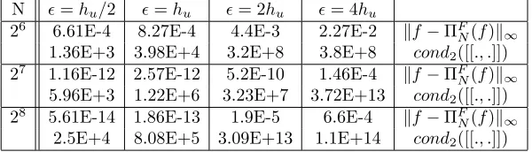
href/2, while for=href the condition number involved in the computation of the Hermitian product weight is too high as table 2 shows, giving results concerning the interpolation property error with respect to the number of discretisation points and to the parameter (), for an analytical functionf(x) = exp(−40(x−(2π/3))2).
N =hu/2 =hu = 2hu = 4hu
26 6.61E-4 8.27E-4 4.4E-3 2.27E-2 kf −ΠFN(f)k∞
1.36E+3 3.98E+4 3.2E+8 3.8E+8 cond2([[., .]])
27 1.16E-12 2.57E-12 5.2E-10 1.46E-4
kf −ΠF N(f)k∞
5.96E+3 1.22E+6 3.23E+7 3.72E+13 cond2([[., .]])
28 5.61E-14 1.86E-13 1.9E-5 6.6E-4 kf −ΠFN(f)k∞
2.5E+4 8.08E+5 3.09E+13 1.1E+14 cond2([[., .]])
Table 2. kf−ΠFN(f)k∞andcond2([[., .]]) as a function of the number of discretisation points
Figure 3. Approximation property for the 1D NUDFT with respect to the solution continuity
with=href/8,=href/4,=href/2,=href, from top left to bottom right.
3.6.
Numerical results for a nonseparable operator
If the operator is nonseparable the operatorP is no longer diagonal.
Exemple 3.7. Let us consider the elliptic problem that follows:
−∇.(a(x, y)∇u(x, y)) =f(x, y) in Ω = [0, π]2,
u= 0 on∂Ω,
with a DD in thex-direction into two overlapping subdomains.a(x, y) =a0+ (1−a0)(1 +tanh((x−(3∗hx∗
y+ 1/2−href))/a))/2, and a0 = 10, a = 10−2, taking into account a jump not parallel to the interface
between subdomains (see Figure 4 (left)). The right hand side f is such that the exact solution is: u(x, y) = 150x(x−π)y(y−π)(y−π/2)/π5. We use a Cartesian grid with 90
×90 elements, uniform inxand nonuniform iny (the maximum distance between the grid points in they-direction is of the order of 2href , (=href/2)).
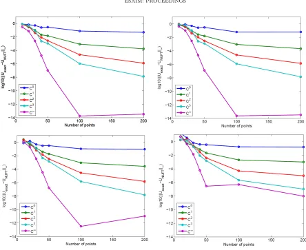
Figure 4 (right) represents Aitken-Schwarz convergence with respect to the Fourier modes kept to build the approximate ˜P[[.,.]] forN∈ {100,200,400}. It exhibits some continuity property with respect to the number of
Figure 4. The function a(x, y) of the test problem, showing the jump not parallel to the interfaces (left). Influence of the approximation ofP[[.,.]] on the interface error convergence for
a strongly nonseparable operator on nonuniform grids (right).
modes does not improve so much the damping factor until reaching the full matrix where the total convergence damping is achieved due to algebraic considerations.
Figure 5 (left) exhibits the convergence of the Aitken-Schwarz method with respect to the number of modes kept to build the reduced matrix ˜P[[.,.]]in accordance to algorithm (2).
Figure 5. Adaptive acceleration using sub-blocks of P[[.,.]], with 100 points on the interface,
overlap= 1, =href/8 and Fourier modes tolerance = ||uˆk
||∞/10i for i = 1.5 and 3 for 1st
iteration andi= 4 for successive iterations (left). Acceleration using sub-blocks of P[[.,.]]with
90 points on the interface, overlap= 5 and=href/2. Top line refers to results in [1] (right).
On the other hand, in Figure 5 (right), the interface is nonuniform with=href/2. It shows good convergence properties even with 10 Fourier modes for the considered problem. The comparison with the result in [1] that considers a uniform mesh and ana priori five diagonal band approximation of theP operator is assumed.
point to build the base. The main idea will be that we can compress the vectorial sequence using a Singular Value Decomposition (SVD). Since the matrixUis built, the matrixP is built the same way.
4.
Approximation compressing the vectorial sequence
A totally algebraic method based on the SVD of the Schwarz solutions on the interface has been proposed when the modes of the error could be strongly coupled [39]. This method offers the possibility for the Aitken Schwarz method to be used on a large class of problem without mesh consideration.
This section focuses on the definition of the orthogonal ”base”Uq. In the following, we use the term ”base” to
denote a set of spanning vectors that defines the approximation space. The key point of these preconditioners’s efficiency is the choice of this orthogonal ”base” Uq. It must be sufficiently rich to numerically represent the
solution at the interface, but it has to be not too large for the computation’s efficiency. Starting from the pure linear convergence Ej =P Ej−1,
∀j ≥1 of the error Ej of the Schwarz DD on the
interface of size n at the iteration j, one can formally build P =
En, . . . , E1 En−1, . . . , E0−1
. But the difficulty can be to invert the matrix
En−1, . . . , E0
which can be close to singular. In a computation, most of the time is consumed solving some noise [40, chapter 8] that does not actually contribute to the solution. The SVD allows us to focus on the main part of the solution.
4.0.1. The singular value decomposition
A singular value decomposition (SVD) of a realn×m(n > m) matrixAis its factorization into the product of three matrices:
A = UΣV∗, (55)
whereU= [U1, . . . , Um] is an×mmatrix with orthonormal columns, Σ is an×mnon-negative diagonal matrix
with Σii =σi,1≤i≤mand them×mmatrixV= [V1, . . . , Vm] is orthogonal. The leftUand rightVsingular
vectors are the eigenvectors ofAA∗and A∗Arespectively. It readily follows thatAvi=σiui,1
≤i≤m
We are going to recall some properties of the SVD. Assume that theσi,1≤i≤mare ordered in decreasing order and there existsrsuch thatσr>0 whileσr+1= 0. ThenAcan be decomposed in a dyadic decomposition:
A=σ1U1V1∗+σ2U2V2∗+. . .+σrUrVr∗. (56)
This means that SVD provides a way to find optimal lower dimensional approximations of a given series of data. More precisely, it produces an orthonormal base for representing the data series in a certain least squares optimal sense. This can be summarized by the theorem of Schmidt-Eckart-Young-Mirsky:
Th´eor`eme 4.1. A non unique minimizer X∗ of the problem minX,rankX=k||A−X||2 = σk+1(A), provided that σk > σk+1, is obtained by truncating the dyadic decomposition of (56)to contain the first k terms: X∗=
σ1U1V1∗+σ2U2V2∗+. . .+σkUkVk∗
The SVD of a matrix is well conditioned with respect to perturbations of its entries. Consider the matrices
A, B ∈ Rn, the Fan inequalities write σr+s+1(A+B) ≤ σr+1(A) +σs+1(B) with r, s ≥ 0, r+s+ 1 ≤ n.
Considering the perturbation matrixE such that ||E||=O(), then|σi(A+E)−σi(A)| ≤σ1(E) =||E||2,∀i.
This property does not hold for eigenvalues decomposition where small perturbations in the matrix entries can cause a large change in the eigenvalues.
This property allows us to search the acceleration of the convergence of the sequence of vectors in the base linked to its SVD.
Proposition 4.2. Let(uk)
1≤k≤q qsuccessive iterates satisfying the pure linear convergence property: uk−u∞= P(uk−1
−u∞). Then there exists an orthogonal base
Uq =
U1, U2, . . . , Uq
of a subset of Rn such that
uk=Pq l=1α
k
lUl,∀k∈ {1, ..., q} with a decrease ofαkl with respect tol for which one can write:
(αk+1
1 −α
k
1, . . . , α
k+1
q −α k q)
t= ˆP(αk
1−α
k−1 1 , . . . , α
k q −α
k−1
q )
where Pˆ def= U∗qPUq. Moreover (α∞1 , . . . , α∞q )t obtained by the acceleration process represents the projection of the limit of the sequence of vectors in the space generated byUq.
Proof. By theorem 4.1 there exists a SVD decomposition of u1, . . . , uq
=UqΣV∗ and we can identifyαkl as σlV∗
kl. The orthonormal property of Vassociated to the decrease ofσl with increasingl leads to a decrease of αk
l with respect to l. Taking the pure linear convergence ofuk in the matrix form, and applyingUq leads to:
U∗q(uk−u∞) =U∗qPUqU∗q(uk−1−u∞) (58)
(αk1−γ1∞, . . . , α
k q−γq∞)
t= ˆ
P(αk1−1−γ
∞
1 , . . . , α
k−1
q −γq∞)
t (59)
where (γ∞
j )1≤j≤q represents the projection ofu∞on thespan{U1, . . . , Uq}.
We can then derive Algorithm 3.
Algorithm 3Vectorial Aitken’s acceleration in the SVD space with inversion
Require: G:Rn
→Rn an iterative method having a pure linear convergence
Require: (uk)
1≤k≤q+2, q+ 2 successive iterates ofGstarting from an arbitrary initial guessu0 1: Form the SVD decomposition ofY =uq+2, . . . , u1
=USVT
2: Setl the index such thatl= max1≤i≤m+1{S(i, i)> tol},{ex.:tol= 10−12.} 3: Set ˆY1:l,1:l+2=S1:l,1:lV1:tl,q−l:q+2
4: Set ˆE1:l,1:l+1= ˆY1:l,2:l+2−Yˆ1:l,1:l+1 5: if Eˆ1:l,1:l is non singularthen 6: Pˆ= ˆE1:l,2:l+1Eˆ1:−l,11:l
7: yˆ∞
1:l,1= (Il−Pˆ)− 1( ˆY
1:l,l+1−PˆYˆ1:l,l){Aitken Formula} 8: u∞=
U:,1:lyˆ∞1:l,1
Proposition 4.3. Algorithm 3 converges to the limitu∞.
Proof. As the sequence of vectorukconverges to a limitu∞then we can write Ξ =
u1, . . . , uq
= [u∞, . . . , u∞]+
E where E is a n×q matrix with decreasing coefficients with respect to the columns. The SVD of Ξ∞ = [u∞, . . . , u∞] leads to have U1 = u∞ and σi(Ξ∞) = 0, i
≥ 2. The fan inequalities lead to have σi(Ξ) ≤
σ1(E) =||E||2, i≥2. Consequently, Algorithm 3 decreases the number of non zero singular values at each loop
iterate.
In Algorithm 3 the building of P needs the inversion of the matrix ˆE1:−l,11:l which can contain very small
singular values even if we selected those greater than a certain tolerance. This singular value can deteriorate the ability ofP to accelerate the convergence. If it is the case, we can proceed inverting this matrix with its SVD, replacing by zeros the singular values less than a tolerance instead of inverting them (see numerical recipes in [13]). A more robust algorithm can be obtained without inverting ˆE−1:l,11:l. It consists in buildingP by applying
the iterative methodG to the selected columns ofUq that appears in Algorithm 3. Then ˆP =U∗1:n,1:lG(U1:n,1:l)
as done in Algorithm 4.
4.0.2. Computation of the Aitken’s acceleration
We now present two improvements of the Aitken’s acceleration algorithm, we first give a criterion to choose the number of snapshots in order to get this burden removed from the user. Second, a generalization of the pseudoinverse by the truncation of small singular values of ˆEn−1 is provided, allowing a more robust Aitken’s
acceleration.
Algorithm 4Vectorial Aitken acceleration in the SVD space without inversion
Require: G:Rn→Rn an iterative method having a pure linear convergence
Require: (uk)
1≤k≤q+2, q+ 2 successive iterates ofGstarting from an arbitrary initial guessu0 1: Form the SVD decomposition ofY =
uq+2, . . . , u1
=USVT
2: Set the indexl such thatl= max1≤i≤q+1{S(i, i)> tol},{ex.:tol= 10−12.} 3: Applyoneiterate of G withl+ 2 initial guessesU:,1:l→W:,1:l=G(U:,1:l) 4: Set ˆP =Ut:,1:lW:,1:l
5: Set ˆY1:l,1:2=S1:l,1:lV1:tl,q+1:q+2 6: yˆ∞
1:l,1= (Il−Pˆ)− 1( ˆY
1:l,2−PˆYˆ1:l,1){Aitken Formula} 7: u∞=
U:,1:lyˆ∞1:l,1
underestimated, but overestimating n leads to perform useless iterations. To avoid overestimating n while performing efficient acceleration we can compute the SVD on the fly during the Schwarz iterations. Thus the acceleration is performed when adding few snapshots does not lead to add columns in ˜U. If ais the number of additional snapshots andS0 the new diagonal matrix containing singular values, then Schwarz iterations are
stopped to perform the acceleration when Eq.(60) is satisfied.
max
i=1...n{i, Sii > S11×F CG}=i=1max...n+a{i, S
0
ii > S110 ×F CG} (60)
To use this adaptive criterion we need to compute the SVD after each addition of snapshots. It can be re-computed from scratch or using the previous SVD thanks to an updating procedure [30, 38]. This updating procedure is called on-the-fly SVD. Since the computational time of the SVD is small relatively to Schwarz iterations, the key advantage of the updating procedure is to reduce the memory requirement: the SVD is truncated after each update, thus ˜U is computed from a U ∈ Rm×(l+a) instead of a U ∈ Rm×n. For large
problems n is usually about twice greater than l+a, and U is the largest matrix involved in the Aitken’s acceleration, furthermoreU is computed on a single processor.
Even with a well computed ˜U, the matrix ˆEn−1 may have very small singular values associated to
approxi-mation errors. These small singular values become the largest ones of ( ˆEn−1)−1 weakening the approximation
of ˆP. Given the SVD ˆEn−1=VEˆ S
†
ˆ
EU T
ˆ
E, and a toleranceξ, we can compute ˆP as:
ˆ
P = ˆEnVEˆ S‡ˆ
EU T
ˆ
E with (S
‡
ˆ
E)ii=
1/(SEˆ)ii if (SEˆ)ii ≥ξ
0 if (SEˆ)ii < ξ
(61)
Unlike the SVD of the snapshots, we cannot use a truncation criterion based on the first singular value because the order of magnitude of this first singular value will decrease from an acceleration to another. Then, we setξ
as the smallest singular value computed before the bend that we observe in the decrease of the singulars values.
5.
Large scale Numerical results
On the macroscopic scale, a porous medium can be described by a model where the solid and the fluid occupy the entire volume. The medium considered here is a parallelepiped domain modelled as a continuum where a representative volume element is larger than the average pore size. For this model of saturated flow in porous media, Darcy’s law and mass conservation law give Eq.(62) where uis the hydraulic head, andK the permeability field.
∇.K∇u=qin Ω
u=α, on Γ1
u=β, on Γ2
∂u
∂n = 0, on∂Ω\(Γ1∪Γ2)
The physical modelling of the heterogeneous media leads to several difficulties even for this linear Darcy equation. The treatment of various scales leads to solving sparse linear systems of very large size, with large condition number because of the heterogeneous permeability fieldK.
5.1.
Highly heterogeneous media
Eq (62) is discretized using a regular grid on which a random permeability field K is generated. This permeability fieldK follows a stationary lognormal probability distribution Y =log(k), which is defined by a meanmY set to zero, and a covariance function
CY(x, y, z) =σ2exp
− "
x
λx 2
+ y
λy 2
+ z
λz 2#
1 2
(63)
where σ is the standard deviation of the log hydraulic conductivity and λx, λy and λz are the directional correlation lengths. To generate the random hydraulic field, a spectral simulation based on the Fast Fourier Transform method [31, 41] is used. For the sake of simplicity, we assume the media to be isotropic: λ=λx=
λy=λz. Then the covariance function becomesCy(r) =σ2(
−r/λ) whereris the distance between two points. Parametersσandλplay a role in the stiffness of the linear system to be solved and in the convergence rate of the Schwarz method. Typically the condition numberκ(A) of the linear system is of the order of magnitude of
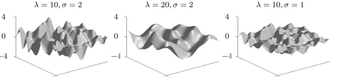
Kmax/Kmin whereKmin andKmax are the minimal and the maximal values of the permeability. An example of a cut of three random permeability fields of 1283 points is given in Figure 6 to illustrate the effect of the parameters. The same random seed is used to generate these three fields.
λ= 10, σ= 2 λ= 20, σ= 2 λ= 10, σ= 1 4
0
−4
4
0
−4
4
0
−4
Figure 6. Values of the permeability in log10 scale for different parameters on a cut atz= 1of
a permeability field of1283 points. Theλparameter plays on the smoothness of the variations, while the parameterσ plays on the scale of the permeability values.
Let us consider a finite volume discretization of a domain Ω that leads to solve the linear system Au=f. Schwarz DD techniques allow us to solve the problem on Ω from the solutions on overlapping subdomains Ωi
such that Ω = SM
i=1Ωi. In the following we assume that a one-directional splitting of Ω is performed: each
subdomain Ωihas at most two neighboring subdomains Ωi−1and Ωi+1. We defineAiuki =f k
i as the local linear
systems of the problem on Ωiat the Schwarz iterationk. The local subdomain solver is the parallel Algebraical
Mutigrid: AGMG of [29].
5.2.
Aitken-Schwarz as a specific solver for three-dimensional groundwater flow problems
5.2.1. Comparison of the approximations ofP
We are now interested in the comparison of both Aitken-Schwarz algorithms in terms of convergence and computational cost. Only the computation of ˆPdiffers between the two algorithms: in algorithm 3 ˆPis computed
as ˆP = ˆEn Enˆ −1
−1
. On the one hand, the computational cost is very low since the dimension of the matrix
ˆ
En−1
is very low. On the other hand, the inversion ofEnˆ −1
can be hazardous because the matrix ˆEn−1
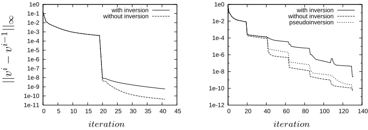
has been approximated. We consider a domain discretized in 1200×4202≈211×106unknowns. The number of snapshots is not chosen adaptively, but fixed to ensure that the acceleration is performed after the same number of Schwarz iterations for both algorithms. This comparison is made for two permeability fields, the first one is generated according to the parameters (λ, σ) = (10,1) and the second one according to (λ, σ) = (20,3). Note that both parameters have been increased in order to slow the convergence rate of the Schwarz method. Convergences are plotted in Figure 7. We remark that convergence are nearly the same for (λ, σ) = (10,1). In that case algorithm 3 is more attractive since the computational is about 27min, instead of 33min for algorithm 4. On the right hand side of Figure 7 we observe that algorithm 3 is less robust than algorithm 4 for stiff problems, but the computation of the pseudoinverse as in Eq.61 clearly improves the robustness.
||
v
i
−
v
i
−
1
||
∞
1e-11 1e-10 1e-9 1e-8 1e-7 1e-6 1e-5 1e-4 1e-3 1e-2 1e-1 1e0
0 5 10 15 20 25 30 35 40 45 with inversion without inversion
1e-12 1e-10 1e-8 1e-6 1e-4 1e-2 1e0
0 20 40 60 80 100 120 140 with inversion
without inversion pseudoinversion
iteration iteration
Figure 7. Error in log scale for (λ, σ) = (10,1) (on the right) and(λ, σ) = (20,3) (on the left)
5.2.2. Weak Scaling test
This implementation has been designed to provide a solution when it is not possible, or not desirable, to compute the solution on the whole problem. The number of subdomains should be as small as possible because the convergence rate of the Schwarz process, and the efficiency of the acceleration, decrease when the number of interfaces increases. Consequently, performing strong scaling tests would consist in increasing the number of processors per subdomain, which is equivalent to compute the strong scaling of the local solver.
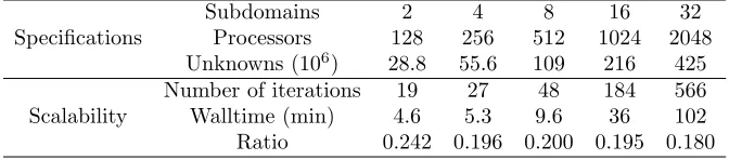
To perform weak scaling tests without taking into account the weak scaling of the local solver, we fix the size of subdomains and the number of subdomains is increased. Algorithm 4 is used since it is the most robust, and the number of snapshots is chosen according to the adaptive criterion. Results are provided in Table 3 where:
• The number of iterations is the total number of Schwarz iterations (Algorithm 4 step 1) needed to reach the convergence.
• The walltime is the running time.
• The ratio is given by the total time per iteration.
Table 3. Weak scaling test: variation of the computational time when the size of the problem is increased, keeping the load per processor constant. The parameters are (λ, σ) = (10,1)
Specifications
Subdomains 2 4 8 16 32 Processors 128 256 512 1024 2048 Unknowns (106) 28.8 55.6 109 216 425
Scalability
Number of iterations 19 27 48 184 566 Walltime (min) 4.6 5.3 9.6 36 102 Ratio 0.242 0.196 0.200 0.195 0.180
the SVD grows faster than the size of ˜P involved in the Aitken’s formula. Performing the SVD itself in parallel could be needed for very large problems.
The number of iterations gives anumerical weak scaling. Notice that the complexity is less than quadratic which is acceptable for this kind of problems. Finally the ratio is nearly constant, so the weak scaling of our implementation well corresponds to thenumerical weak scaling.
6.
Conclusions
We showed the importance to represent cheaply the solution of the Schwarz DD method at the artificial interface generated by the domain decomposition. These solutions contain enough information in order to accelerate the convergence of the iterative method to the searched solution. The approximation space should be sufficiently rich to represent the searched solution. The nonuniform Fourier tansform allowed to develop an adaptative acceleration which gave us an estimate on the convergence for each Fourier-like mode. This allows us to select the modes that are involved in building the error operator P on the interface. However, this nonuniform Fourier approximation is dependent on the regularity of the searched solution at the artificial interfaces. This is why the singular value decomposition of the iterated solutions provides a more general tool to build the approximation space. It still has the two major properties: an orthogonal ”basis” to generate a vectorial subspace and a decreasing of the coefficients relative to this ”basis” involved in the decomposition of the solution. This last property gives an estimate for the selection of the modes involved in the building ofP. Then we succeed in performing large scale computing on problem of sizes that cannot be handled by the local (subdomain) solvers.
Some extensions of this methodology have been applied as preconditioning techniques for the Krylov solver. This is based on the acceleration of the Restrictive Additive Schwarz by Aitken with a Richardson formulation [10] [9]. Some illustrations of ill conditioned problems arising from computational fluid dynamics field can be found in [11].
This methodology can also be applied to time DD [23]. Some extensions to nonlinear problems are under consideration. In this case some use of the-topological algorithm of [6] can replace the Aitken’s acceleration of the convergence technique [21]. Another issue is to consider some nonlinear transmission conditions that makes the convergence of the Schwarz DD purely linear in a transformed space (with a nonlinear change of variable) [22].
Aknowledgement
The author thanks one referee for pointing out many useful corrections for the readability of this paper.
References
[1] J. Baranger, M. Garbey, and F. Oudin-Dardun. The Aitken-like acceleration of the Schwarz method on nonuniform Cartesian grids. SIAM J. Sci. Comput., 30(5):2566–2586, 2008. ISSN 1064-8275. . URL
![Figure 2. Steps to build the P[[.,.]] matrix](https://thumb-us.123doks.com/thumbv2/123dok_us/10072364.1993653/13.612.122.439.320.453/figure-steps-to-build-the-p-matrix.webp)