Allocating Fixed Costs: A Goal Programming Model Based on Data Envelopment Analysis

(1)

Available online at http://ijdea.srbiau.ac.ir

Int. J. Data Envelopment Analysis (ISSN 2345-458X)

Vol.7, No.3, Year 2019 Article ID IJDEA-00422, 10 pages Research Article

Allocating Fixed Costs: A Goal Programming

Model Based on Data Envelopment Analysis

S. Asghariniya1, S. Mehrabian*2, H. Zhiani Rezai3

(1,2) _{Department of Mathematics, Faculty of Mathematical Sciences and Computer,} Kharazmi University, Tehran, Iran

(3) _{Department of Mathematics, Islamic Azad University, Mashhad Branch, Mashhad, Iran}

Received 29 January 2019, Accepted 17 May 2019

Abstract

Most organizations consist of several individual units. Resource allocation issue appears when requiring to determine an equitable share of costs for these independent units. Data Envelopment Analysis has been proved as a useful technique to solve allocation problems. This paper presents a linear programming model based on DEA methodology to find an equitable allocation. To compare obtained results, we use the proposed model to a data set of prior studies.

Keywords: DEA, Fixed Cost Allocation, Linear Programming, Goal Programming.

1. Introduction

Today the most organizations (e.g. banks and insurance institutes) consist of the various units which under the control of the main organization (unified management) act independently. Sometimes the manager presents some

*. Corresponding author: Email: [email protected]

(2)

24

share is raised. Answering this problem has the great importance from both economic and management perspectives so many researches have been done regarding this issue. Due to particular properties of DEA, there were several attempts in recent years to solve allocation issue by using this methodology. DEA is a non-parametric method for evaluating the independent decision making units which was presented for the first time by Charnes et al. [6]. In this method each decision making unit is recognized by the input and output vectors. For evaluation, the ratio of the weighted sum of outputs to the weighted sum of inputs is recognized as efficiency score. In this method weights are determined such that the relative efficiency score of under evaluation unit becomes the maximum value which is possible. Aftermath, this method has widely been used by scholars in various areas. One of these areas is to utilize DEA for solving the fixed cost allocation problem. Fixed cost allocation problem illustrates how to determine a fair share of a total cost for some decision making units which acts independently under the control of the unified management.

Athanassopoullos [2] attempt to solve allocation issue via a goal programming model. To find an equitable allocation, they used Russell model and changed it to an aggregated goal programming model. Cook and Kress [7] addressed the allocation problem using DEA. In order to achieve a proper allocation, they considered the allocated cost to each unit as a new input and then determined the proper amount through solving various linear programs. In their proposed method, the allocation was determined in such a way that the efficiency of units was preserved after allocation. Cook and Zho [8] developed this method from CCR model [6] into BCC model [3] and from input orientation into output orientation. Lin [12] claimed that the presented method by Cook and Zho [8] is not a

comprehensive method and through imposing specific limitations on this method the obtained solution will not result in feasible solution. He added some fixed target to the model in order to improve this condition and to obtain a feasible allocation. In other article Lin [13] replaced minimal deviation principle with efficiency invariance assumption in the article of Cook and Kress [7].

Beasley [4] presented a different method. After considering the share of each unit as a new input, he used a non-linear model based on DEA. In this model, he utilized a common set of weights and according to what was mentioned in the article, he used several other models to get a unique solution. Based on Beasley [4], Kordrostami and Amirteimoori [1] presented other method in which with efficiency invariance assumption the proper allocation was obtained. In their method, several other models should also be solved in order to get a unique allocation. Jahanshahloo et al. [10] showed the efficiency invariance assumption is not a necessary constraint in Kordrostami and Amirteimoori [1]. They also preposed two approaches to obtain a fixed allocation based on efficiency invariance and common set of weights principles.

Li et al. [11] attempted to obtain a fair allocation considering the allocated cost to each unit as the extra input. They assumed that each DMU has other costs which are considered as an input for them and then the share of each DMU from the fixed cost is added to the input. This method was also assumed the efficiency invariance constraint.

(3)

S. Asghariniya, et al. / IJDEA Vol.7, No.3, (2019), 23-32

25

first stage and its cross-efficiency score in the next stage (using the obtained weights from the obtained linear model) were considered. In each iterative process, they determined the share of each unit which was obtained from the linear model of the K stage with the condition

1

k k

e e .

Articles published in this area can be divided into the three general categories: 1) Articles which used the common set of weights in order to find proper allocation. 2) Articles which used iterative methods for the abovementioned purpose.

3) Articles which solved non-linear models for determining proper share. The presented method in this article on the contrary of the prior studies belongs to none of these three groups. In this article a linear model presents for solving the allocation problem using particular weights instead of the common set of weights. It should be mentioned that the presented model is not a duplication of other models and the optimal solution is achieved by solving just one linear programming problem.

The article is organized as follows: section 2 describes briefly the basic CCR model. In section 3 a model is presented for simultaneous evaluation of units. Section 4 deals with the analysis and solving the model. Finally, the conclusion of the article is provided in section 5.

2. The basic model

In this section we briefly describe the traditional DEA method to evaluate decision making units (DMUs). Let us consider a set of n decision making units; each of them produces the output vector

j

y (yt_j (y₁_j, ,y_sj)) consuming the input vector

j

x (xt_j (x₁_j, ,x_mj)). For evaluating each decision making unit, the input and output weights of under

assessment units are determined in such a way that the relative efficiency reaches the maximum. To this end, the fractional model (1), called the input orientation model, is utilized. This model was introduced by Charnes and Cooper [5].

Max

. . 1, 1, ,

,

p p p

p

p p

p

s m

j p

j

s t j n

1 1

u y

v x

u y

v x

u v

(1)

In model (1) 1_s and 1_m mean row vectors with s and m members of 1, respectively.

The row vectors up (u₁p, ...,u_sp) and

1

( ,...,p _mp)

p _v _v

v are unknown weights

corresponding to outputs and inputs, respectively. The superscript p indicates the weights are determined by under assessment unit DMUp in order to obtain the maximum efficiency score. in two ending constraints of the model (1) is a non-Archimedean number and guarantees the weighted vectors are strictly positive. In fact, when evaluating each unit it is not possible to ignore none of its inputs or outputs.

(4)

26 Max

,

. . 1

0, 1, ,

p p j j p p p p p p s m s t j n 1 1 u y v x

u y v x

u v

(2)

From the first constraint and the second set of constraints (for j=p) it is concluded that

1

p p

u y . Then, according to the goal programming, model (3) can be replaced instead of model (2):

, Min 1 0 . . 1

0, 1, , , p p p p p p p p p p

s m p

j j n n n s t j n 1 1 u y v x

u y v x

u v

(3)

If we simultaneously consider constraints in model (3) for different DMUs (i.e. p=1,…,n) it will be seen that the constraints related to one DMU are not dependent to another one. So the optimal solution for all DMUs obtained of n time solving model (3), can be obtained of solving model (4) in one time (see theorem1).

1 Min

. . 1, 1, ,

n p p p p p n

s t u y n p n

1, ,

0

1 , 0 1, , ,

, p p p p s m p p p j j p n p n

n p n

j n

1 1

v x

u y v x

u v

(4)

Theorem1: If

1

1_{, ,} _, 1 _{, ,}

(u un v vn ,n , ,n_n) is an optimal solution of model (4), then

* ) * *

, ,

(uk vk n_k is an optimal solution of model (3) for DMUk (k {1, 2, , }n ) and vice versa.

Proof: At the first, suppose that

1 1 _{, ,} _, 1 _{, ,}

(u un v vn ,n , ,n_n) is an optimal solution of model (4). In contradiction, suppose that there exists a k

that (uk ,vk ,n_k) is not optimal solution of model (3) in assessment DMUk. Thus it

has a feasible solution (uk,vk,n_k) with objective valuen_k n_k*. Now, because of the set of constrains connected with each DMU are independent each of them, so

1_{, , , ,} 1

(u uk u vn , , ,vk, ,vn, , , , , )n₁* n_k n_n is a feasible solution of model (4), with objective value

1

p k

n p

p kn n p n

that is a contradiction. So If

1 1

1

( , , n , , , n , , , )

n

n n

u u v v is an

optimal solution of model (4), then

(uk ,vk ,n_k) is an optimal solution of model (3) for each DMUk (k {1,2, , }n ).

Next, suppose that (uk ,vk ,n_k) is an optimal solution of model (3) in assessment DMUk (k {1, 2, , }n ), we proof that (u1, ,un ,v1 , ,vn ,n₁, ,n_n)

is an optimal solution of model (4). Suppose that in contradiction, model (4) has a feasible solution such as

1 1

1

( , ,u u vn, , ,vn, , ,n n_n) with objective value

1 p_k 1

n n

p

p n p n . In this case,

there exists at least one k with

k k

n n .

(5)

27

(3). This contradiction proves

1

1 _{, ,} _, 1_{, ,}

(u un v vn ,n , ,n_n) is an

optimal solution of model (4).

However the number of constraints of model (4) is more than model (3), this model enjoys two main advantages. First of all, in evaluation of units where number of them is small, utilization of model (4) ,because of solving just one model, takes less time than solving model (2) n times. The second advantage of model (4), which constitutes the aim of this paper, is that the proposed model allows us to simultaneously impose some constraints on all units or the related weights.

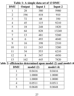
3.1. Example

With the help of a simple example the abovementioned claim can easily be approved. Consider a data set which

involves thirteen DMUs each of them has two inputs and one output (Table 1). Table 2 shows the efficiencies of units obtained by model (2) and (4).

In the second column of Table 2 the efficiency of each unit is calculated by the optimal value of the objective function of

model (2) i.e. p* p

u y and efficiencies of column three was achieved by model (4)

and using 1 n*_p formula. As it can be seen in the table, these values are equal but what is considerable is that the needed time for determining the efficiency of all units with help of mdoel (2) and (4) and using GAMS Software is 0.316 and 0.016, respectively, which clearly indicate that the time spent by model (4) is less than the time spent by model (2).

Table 1: A simple data set of 13 DMU

DMU Output Input 1 Input 2

1 28 380 5980

2 196 418 910

3 72 68 350

4 45 115 9210

5 18 248 1820

6 64 828 13240

7 13 481 5260

8 6 493 4040

9 16 198 2310

10 11 243 3280

11 34 553 6210

12 8 347 4950

13 162 445 7820

Table 2: efficiencies determined upon model (2) and model (4)

DMU model (2) model (4)

1 0.0416 0.0416

2 1.0000 1.0000

3 1.0000 1.0000

4 0.0511 0.0511

(6)

28

6 0.0010 0.0010

7 0.0184 0.0184

8 0.0098 0.0098

9 0.0665 0.0665

10 0.0341 0.0341

11 0.0385 0.0385

12 0.0149 0.0149

13 0.1537 0.1537

4. Allocation Problem

This section deals with allocation problem using the proposed linear model. To this end, consider an organization which consists of n individual subsections. Suppose that the main management spent F total cost to benefit all units. The share of unit j of F is shown by

j

f

whereas

1 n

j j

f F. Give the share of unit j (i.e.

f

j) as a new input for it. Since the aim is a fair allocation, the weight of the new input is assumed equal for all units. Next, with a small change in model (4), model (5) is achieved.

1

Min

. . 1 , 1, ,

1 , 1, ,

0

1, , , 1, ,

, , 1, ,

, 0 , 1, ,

0 n p n p p p p p p p p p p

j j j

p p p s m p f p n

s t n p n

kf p n

kf

j n p n

F

p n

n p n

k

f

1 1

u y

v x

u y v x

u v

(5)

In model (5) multiple k is the weight of the new input ((m+1)th input) of units. The both 5th constraint and the 6th set of constraints in model (5) come from the condition of allocation problem. It should paid attention that model (5) is a non-linear model but it can be converted to the liner

model (6) through replacing p

kf with ' p

f in connected constraints.

1

' 1 Min

1 1, ,

' 1 , 1, ,

' ₀

1, , , 1, ,

, , 1, ,

' ₀ _, _{1, ,}

0 . . , , n p n p p p p p p p p p p p

j j j

f

p p

s m

p p

n

n p n

f p n

f

j n p n

kF

p n

f n p n

k

s t

1 1

u y

v x

u y v x

u v

(6)

The aim of solving model (6) is to find optimal allocation but what is achieved

from model (6) are f_j' s, although based on the changes made in order to achieve

model (6) we have '

j j

f kf , so j

f can be obtained from the equation f_j f_j'/k.

4.1. Numerical Example

(7)

29

twelve DMUs which each of them

have three inputs and two outputs. The purpose is to allocate the fixed cost F=100 to units. The results of allocation based on models of [3, 7, 9] as well as the presented model in this paper can be observed in Table 4.

The second, third and fourth columns of table 4 show the share determined for each

DMU by the aforementioned models which were derived from related articles. The last column shows the results achieved by performing model (7) by the GAMS software with considering 𝜀 =

0.0001 and using the final formula

' _/

j j

f f k.

Table 3: Data set of Cook and Kress [7] paper

Output2 Output 1 Input 3 Input 2 Input 1 DMU

751 67 9 39 350 1

611 73 8 26 298 2

584 75 7 31 422 3

665 70 9 16 281 4

445 75 6 16 301 5

1070 83 17 29 360 6

457 72 10 18 540 7

590 78 5 33 276 8

1074 75 5 25 323 9

1072 74 6 64 444 10

350 25 5 25 323 11

1199 104 6 64 444 12

Table 4: Allocated cost to DMUs obtained by different methods

DMU Cook and Kress [7] Beasley [4] Du (2013) Presented model(6)

1 14.52 6.78 5.79 4.7259

2 6.74 7.21 7.95 8.6618

3 9.32 6.83 6.54 8.5787

4 5.60 8.47 11.10 9.2550

5 5.79 7.08 8.69 11.5954

6 8.15 10.06 13.49 5.9536

7 8.86 5.09 7.10 7.7072

8 6.26 7.74 6.83 10.5076

9 7.30 15.11 16.68 12.3794

10 10.08 10.08 5.42 7.8698

11 7.30 1.58 0 0.0000

12 10.08 13.97 10.41 12.7656

sum 100 100 100 100

To compare the aforementioned methods and the presented method in this article, data in table 5 should be considered. The second column of this table shows the efficiency of units before allocation and other columns display the efficiency of units after allocation of the determined

share (by each method) as the fourth input for each DMU. The efficiencies were calculated with the help of GAMS Software and with considering 0.0001

.

(8)

30

In this paper, we have shown that just one linear programming model is sufficient to evaluate all DMUs. Based upon proposed LP, we present a model for allocating fixed costs. The results have been compared with some of previous approaches to show

the concordance of our presented approach. With a few changes, the proposed approach in this article is useful for resource allocation and target setting. Also using suitable changes it is usable for BCC model.

Table 5: Efficiencies before and after allocating

DMU Primary Efficiencies Cook (1999) Beasley [4] Du (2013) presented model (6)

1 0.7560 0.7555 1.0000 1.0000 1.0000

2 0.9223 0.9222 1.0000 1.0000 1.0000

3 0.7152 0.7152 0.9948 0.9949 1.0000

4 1.0000 1.0000 1.0000 1.0000 1.0000

5 1.0000 1.0000 1.0000 1.0000 1.0000

6 0.9602 0.9602 1.0000 1.0000 1.0000

7 0.8426 0.8424 1.0000 1.0000 1.0000

8 1.0000 1.0000 1.0000 1.0000 1.0000

9 1.0000 1.0000 1.0000 1.0000 1.0000

10 0.8242 0.8241 1.0000 1.0000 1.0000

11 0.3325 0.3325 1.0000 1.0000 1.0000

(9)

31

References

[1] Amirteimoori A.R., and Kordrostami, S., “Allocating fixed costs and target setting: A dea beased approach”, Applied Mathematics and Computation, 171 (2005), 136-151.

[2] Athanassopoulos, A.D., “Goal programming and data envelopment analysis (GoDEA) for target-based multi-level planning: Allocating central grants to the Greek local authorities”, European Journal of Operational Research, 87 (1995), 535-550.

[3] Banker, R.D., Charnes A., and Cooper, W.W., “Some models for estimating technical and scale inefficiency in data envelopment analysis”, Management Science, 30 (1984), 1078-1092.

[4] Beasley, J.E., “Allocating fixed costs and resources via data envelopment analysis”, European Journal of Operational Research, 147 (2003), 197-216.

[5] Charnes, A., and Cooper, W.W., “Programming with linear fractional functions”, Naval Research Logistics Quarterly, 9 (1962), 181-186.

[6] Charnes, A., Cooper, W.W., and Rhodes, E., “Measuring the efficiency of decision making Units”, European Journal of Operational Research, 2 (1978), 429-444.

[7] Cook, W.D., and Kress, M., “Characterizing an equitable allocation of shared costs: a DEA Approach”, European Journal of Operational Research, 119 (1999), 652-661.

[8] Cook, W.D., and Zho, J., “Allocation of shared costs among decision making

units: a DEA approach”, Computer and Operations Research, 32 (2005), 2171-2178.

[9] Du, J., Cook, W.D., Liang, L., and Zhu, J., “Fixed cost and resource allocation based on DEA cross-efficiency”, European Journal of Operational Research, 235 (2014), 206-214.

[10] Jahanshahloo GM, Sadeghi J, Khodabakhshi M (2017) Proposing a method for fixed cost allocation using DEA based on the efficiency invariance and common set of weights principles. Mathematical Methods of Operations Research 85(2):223-240

[11] Li, Y., Yang, F., Liang, L., and Hua, Z., “Allocating the fixed cost as a complement of other cost inputs: A DEA approach”, European Journal of Operational Research, 197 (2009), 389-401.

(10)