http://jbe.tums.ac.ir
Please cite this article in press as: Ghanbari A, YekaninejadMS, PakpourA, SanjariS, NourijelyaniK. Comparison of the accuracy of beta-binomial, multinomial, dirichlet-multinomial, and ordinal regression in modelling quality of life data. J Biostat Epidemiol. 2018; 4(2): 61-71
Original Article
Comparison of the accuracy of beta-binomial, multinomial, dirichlet-multinomial, and ordinal regression in modelling quality of life data
Ali Ghanbari1, Mir Saeed Yekaninejad1*, Amir Pakpour2, Sobhan Sanjari1, Keramat Nourijelyani1
1 Department of Epidemiology and Biostatistics, School of Public Health, Tehran University of Medical Sciences, Tehran,
Iran
2 Social Determinants of Health Research Center, Qazvin University of Medical Sciences, Qazvin, Iran
ARTICLE INFO ABSTRACT
Received 21.01.2017 Revised 09.08.2017 Accepted 05.11.2017
Background & Aim: Questionnaires are used mostly as a tool in medical research. Due to the different varieties of questionnaires, we may face different score distributions. In many cases multiple linear regression assumptions are violated. Beta-binomial regression model has the high flexibility and compatibility with this situation. In previous studies there were no comparison between beta-binomial accuracy and other models to fitting quality of life data. So in this study, our aim is to compare the accuracy of models to prediction.
Methods & Materials: In this cross-sectional study we collected the quality of life data from 511 healthy women in Qazvin, Iran. The data were used to compare accuracy of beta-binomial model and with some other models. Since beta-beta-binomial considers the discrete response variable, so it should be compared with other similar models which are mostly used such as multinomial, dirichlet-multinomial and ordinal regression models. The main method that we used in our study was cross-validation to determine the accuracy of different models. To compare the different aspects, vast variety of situations were made and considered.
Results: Regarding to the accuracy of models that were obtained by cross-validation in different situations, beta-binomial model had better accuracy among all models.
Conclusion: According to the results, we have concluded that beta-binomial model is more accurate in prediction and fitting to the quality of data than the other models. The main advantages of this model are its simplicity, more efficacy and accuracy than the similar models.
Key words: Regression analysis; Survey;
Questionnaire; Quality of life; Woman; Statistical model
Introduction
Questionnaires are among the most widely and extensively used tools in medical research, and so far various questionnaires are designed and applied. HRQOL (Health-related quality of life) questionnaires are of a particular importance (1). As a result of this diversity, we also see variation in the distribution of variables, which is challenging in terms of analysis. Analysis of data from quality of life questionnaires is no exception (2-4). For example, most of the scores came from this type of questionnaire are bounded and highly skewed,
and usually because the final score is obtained from the sum of several questions, each of which has multiple options with certain numerical values, consideration of the final scores with continuous nature is worth a major attention. In order to consider the continuity nature, diversity of number of unique scores must be high. When the number of response classes is more than 7, it can be treated continuously and ordinally (5), and it is not so interesting to deal with a substantial discrete variable, continuously, because it will lead to some problems in fitting of continuous models. On the other hand, another noteworthy issue is the consideration of the type of response variable, which in most cases, scores are ordinally (6).
Up to now, many models have been considered for analyzing various kinds of
_____________________________________________________
* Corresponding Author: Mir Saeed Yekaninejad, Postal Address: Department of Epidemiology and Biostatistics, School of Public Health, Tehran University of Medical Sciences, Tehran, Iran.
questionnaires, including quality of life, so that for a specific data, and to achieve a goal, several models can be fitted. The important point is to use the model(s) that has the highest accuracy along with simplicity and interpretability. For the scores derived from quality of life questionnaires, we can also fit different models, including models that consider the response variable to be continuous and discrete.
One of the most widely used methods to investigate the effect of several variables on a response variable is the multiple linear regression. This method has several assumptions that must be met. One of which is that the response variable should be continuous and with a normal distribution. Sometimes the response variable does not meet these conditions and such situation is not uncommon. Being a bounded response variable is also another problem in this context. Sometimes, methods that require that the response variable has a normal distribution with a constant variance are unsuitable for analysis (5-7). Sometimes the variation of the unique score of the response variable resulting from the questionnaire is small, which itself is a reason to pass up the idea of response variable is continuous. These conditions are just examples of the situation where the score from the questionnaire (which is supposed to be the response variable), do not meet the assumptions of the multiple linear regression model .If the violation of assumption is significant, it may cause problems such as lack of validity in results. Multiple linear regression results are not very reliable when data are skewed (6,8). It has been shown that using multiple linear regression models to fit these kinds of data has great weaknesses, including its inability to identify effective independent variables. if dependent variable is not continuous, this model is not applicable and the results may be significant although clinically not meaningful (9).
Ordinal regression including odds proportional has been proposed for analysis of these kinds of data (3,5). Ordinal regression is suitable for cases where the response variable is essentially ordinal (5), but not applicable for occasions that they are more continuous (10). This model is suitable for the response variables with the smaller number of categories, and as the number of categories increases, the interpretation of the model results become difficult. Different dimensions of quality of life questionnaires have
a considerable variety of unique value of scores. For example, a dimension may have 5 unique values and other dimension has 30 unique values. Clinically, it is important to fit and apply the same model to different dimensions. Beta-binomial regression does not have the limitations like the ordinal regression in fitting different dimensions which are different in the variety of unique data, and this itself is a very important reason for the suitability of a beta-binomial model (6,11). Some dimensions of quality of life questionnaire are substantially discrete, and fitting the models that consider the discrete-response variable to be discrete are more appropriate than those that consider the response variable to be continuous (6). If continuous models, such as tobit regression and binomial-logit-normal regression are used, the beta-binomial regression is more appropriate in terms of the interpretation and meeting the assumptions in fitting the SF-36 data (11).
In this study, we focus more on the statistical aspect than clinical aspect which is the difference with previous studies. We compare Beta-Binomial (BB) with Multinomial (MU), dirichlet-multinomial (DM), multiple linear regression (ML) and ordinal proportional odds (OR) models in terms of accuracy using cross-validation.
Methods
SF-12 questionnaire is consisting of two subscales, the mental component summary and the physical component summary. Since the Physical Component is far from the multiple linear regression assumptions in our data so it is more appropriate. The aim of this study was to evaluate the goodness of fit of mentioned models on physical Component of quality of life data. Four models are discrete-response variables. The multiple linear regression model was only fitted (since it does not perform well in our response variable conditions) to show its weakness in fitting.
Data
http://jbe.tums.ac.ir
63
welfare), therefore we restricted our research to physical responses. In all cases, participants’ consents were obtained. Also our focus is on response variable SF-12 questionnaire’s physical aspect and other are predictor variables. SF-12 and HADS questionnaires validity and reliability were assessed in Iran (12, 13).
Categorizing response variable
As we indicated, our response variable is continuous, but in our models, except multiple linear regressions, the response variable must be discrete. One of the challenges ahead is to convert the response variable from continuous to discrete. Choosing different methods to classify the response variable may affect the results of the models. To reduce the effect of different classifying the response variable on the results of the models, we classify the variable of the response in different ways, and for each classification, we fit the models separately. To classify the response variable, eight different modes were considered, which will be discussed in the following.
There are two factors in classification. The first factor is the number of classes and the second factor is the way we choose the cut points to classify the response variable. Having these two factors means that we face different scenarios for classification of response variable. The number of categories were considered three to six. We apply two different methods to determine the cut points. In the first one, the cut points were determined equal in a way that the length range of the response variable is divided by the cut points into equal intervals. And the second is to specify the cut points based on equal percentiles, which means cut points are determined in a way that the number of observations in each class is approximately equal. In case of equal percentiles, the length of the intervals may not be equal and some of the cut points may be close together.
Comparing Criteria
With eight different categories, we control the categorization effect. Two methods were used. The first one is to compare the AIC (Akaike information criterion) values and the second is the cross-validation method. We fit five models for each of the eight different scenarios and then calculate the values of AIC for models. The following is a description of the
cross-validation method.
In the cross-validation method, a section of data was selected as the training set, and based on these data, the models were fitted, and then using these models we predict the response variable of the test data set (the remaining data). Given that the response variable is discrete, the accuracy of the models is calculated by the percentage of test data set observations that their class is correctly predicted by the fitted model from the training set.
In the cross-validation method, some matters should be contemplated. The first thing is that what percent of the original data should be chosen as a training set. This could affect the accuracy of the models, so to eliminate this effect; different scenarios for choosing the percentage of training set from the main data were studied. Selective percentages are 30, 40… 80 and 90, so for each of the 8 different scenarios, we will consider four different percentages for choosing the training set. So far, a total of 32 different scenarios for comparing models were brought up.
Another issue is how to choose the training set, here the choice of training set is taken from the original data randomly. To eliminate effect of random selection of training set, we repeat this procedure 1000 times. Therefore, for every specific response category, types of determining cut points and percentage training set, we have 1000 accuracy for 5 models.
used from R libraries.
Results
The descriptive information of the response variable which has been scaled between zero and 100 and other variables as independent variables are shown in Table 1. Also, in figure 1, the histogram of the response variable is plotted which is quite skewed.
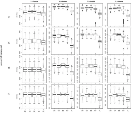
In each of the 32 scenarios for each model, we have 1000 model accuracies, which the box plot of them divided into 32 scenarios in the form of two figures. In figure 2, 16 different scenarios, equal intervals method (the choice of cut points are based on equality of intervals) with four different scenarios for the number of response variable classes (three to six classes), and four different percent for selecting the training set from the main data (left side of figure). Figure 3 is exactly like figure 2, with the difference of choosing cut points is based on equal percentiles.
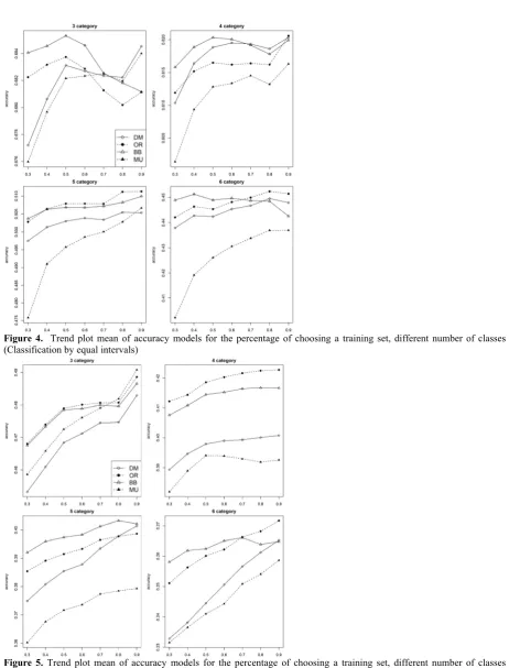
Figures 4 and 5 were drawn to investigate the effect of choosing a training set percentage on the accuracy of models. In each plot, horizontal axis is the percentage of the training set from the
main data. The vertical axis represents the accuracy of the model as the percentage of correct prediction made by the model. Every model is drawn up as a Different pattern in each figure. The average of the accuracy of the models is specified in each choice of training set and linked together to examine the trend.
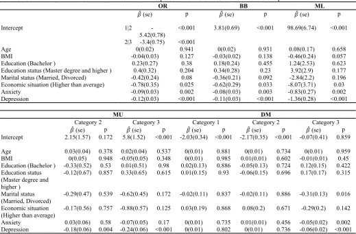
In Table 2, coefficient estimation and p-values of independent variables for models are presented only for the scenario where the response variable is classified into four classes with equal intervals. In Table 3, the AIC values obtained from fitting the models were shown. According to the AIC criteria in Table 3, we find that in each model, the higher the number of response variable classes, the greater the AIC value. When the number of the classes is specified, AIC value is greater when cut points are chosen by equal percentiles method rather than by equal intervals. As a result, the higher the number of classes, the greater the AIC value. Also the method for choosing cut points based on equal intervals gives less AIC value than equal percentiles, which indicates that the model is better. Due to the AIC criteria, number of classes and classification method are effective in
Table 1. Descriptive statistics of dependent and independent variables
Mean SD Min Max
Quality of Life – Physical component 73.92 23.01 0 100
Age 26.32 6.59 15 62
BMI 22.86 4.07 14.88 39.44
Anxiety 8.87 4.76 0 21
Depression 6.53 4.62 0 21
Category Frequency Percent
Education level Non academic 92 18
Bachelor 279 54.6
Master degree and higher 140 27.4
Economic status Average and lower than average 476 93.2
Higher than average 35 6.8
Marital status Single 191 37.4
Married, Divorced 320 62.6
Figure 1. Histogram of response variable (quality of life from physical point of view) Physical score SF-12
F
req
uency
0 20 40 60 80 100
0
50
100
http://jbe.tums.ac.ir 65
fitting the models.
Discussion
In the study of Arostegui et al. (11), who investigated the eight models, multiple linear regression, with least square and bootstrap estimations, to bit regression, ordinal logistic and probit regressions, beta-binomial regression, binomial-logit-normal regression and coarsening in fitting the quality of life questionnaire (SF-36 questionnaire), there are also conditions such as severe skewness, being bounded, low diversity, and ignoring continuity and non-normality of the response variable. When it comes to factors such as good interpretability, the ability of the model to distinguish variables that are clinically
meaningful and simplifying the model, the beta-binomial regression model was recognized as a good model. The superiority of beta-binomial regression in fitting quality of life data, compared with multiple regression are shown in another study (6). Also, the beta-binomial regression model gives satisfactory results in many conditions (11). In an article, the scores of quality of life questionnaire are suited well to the beta-binomial distribution (8). Beta-Binomial regression is a valid method for analyzing quality of life scores (11). The beta-binomial regression model is more appropriate than multiple linear regression analysis for analyzing quality of life questionnaires, not only because of identifying meaningful independent variables,
Table 2. Coefficients of fitted models for the case where the response variable is divided into three classes of equal intervals.
OR BB ML
(se) p (se) p (se) p
Intercept 1|2
-5.42(0.78)
<0.001 3.81(0.69) <0.001 98.69(6.74) <0.001
2|3 -3.4(0.75) <0.001
Age 0(0.02) 0.941 0(0.02) 0.931 0.08(0.17) 0.658
BMI -0.04(0.03) 0.127 -0.03(0.02) 0.138 -0.46(0.24) 0.057
Education (Bachelor ) 0.23(0.27) 0.38 0.18(0.24) 0.455 1.24(2.53) 0.623
Education status (Master degree and higher ) 0.4(0.32) 0.204 0.34(0.28) 0.23 3.92(2.9) 0.177
Marital status (Married, Divorced) -0.42(0.24) 0.08 -0.36(0.21) 0.092 -2.84(2.2) 0.196
Economic situation (Higher than average) -0.78(0.35) 0.025 -0.62(0.29) 0.033 -8.07(3.71) 0.03
Anxiety -0.09(0.03) 0.002 -0.08(0.03) 0.003 -0.83(0.27) 0.002
Depression -0.12(0.03) <0.001 -0.11(0.03) <0.001 -1.36(0.28) <0.001
MU DM
Category 2 Category 3 Category 1 Category 2 Category 3
(se) p (se) p (se) p (se) p (se) p
Intercept 2.15(1.57) 0.172 5.8(1.52) <0.001 -2.03(0.34) <0.001 -2.17(0.35) <0.001 -0.07(0.41) 0.859
Age 0.03(0.04) 0.378 0.02(0.04) 0.537 0(0.01) 0.881 0(0.01) 0.734 0(0.01) 0.959
BMI 0(0.05) 0.948 -0.05(0.05) 0.348 0(0.01) 0.985 0.01(0.01) 0.602 -0.01(0.01) 0.45
Education (Bachelor ) -0.33(0.52) 0.53 0.01(0.51) 0.98 0.02(0.13) 0.886 -0.05(0.13) 0.724 0.12(0.15) 0.422 Education status
(Master degree and higher )
-0.12(0.67) 0.857 0.33(0.65) 0.615 0.01(0.15) 0.93 -0.06(0.15) 0.696 0.17(0.17) 0.315
Marital status (Married, Divorced)
-0.29(0.47) 0.539 -0.62(0.45) 0.172 -0.02(0.11) 0.837 -0.02(0.11) 0.886 -0.31(0.13) 0.016
Economic situation (Higher than average)
-0.17(0.56) 0.757 -0.88(0.57) 0.125 0.03(0.19) 0.868 0.08(0.2) 0.671 -0.29(0.2) 0.142
Anxiety 0.03(0.06) 0.58 -0.07(0.05) 0.17 0(0.01) 0.735 0.01(0.01) 0.456 -0.05(0.02) 0.002 Depression -0.18(0.06) 0.004 -0.24(0.06) <0.001 0(0.01) 0.802 0(0.01) 0.736 -0.06(0.02) <0.001
Table 3. AICs obtained from fitting of the models for situations in which the response variable varies from 3 to 6 classes, each mode being divided by equal distances and equal percentages
Equal distance Quantile distance
3 category 4 category 5 category 6 category 3 category 4 category 5 category 6 category
OR 721 960 1213 1372 1029 1304 1485 1738
BB 997 1575 1902 2083 1409 2279 2813 2780
MU 732 979 1244 1418 1033 1312 1498 1766
DM -8017 -12964 -18215 -23784 -7824 -12785 -18117 -23668
but also because of measuring the relationship between independent and dependent variables from a clinical point of view (9).
We examined the models in different situations. Now, let's look at which models in comparison with other models have better fit, and how models behave in different situations that we have identified.
We will continue to compare the models from the cross-validation point of view. In figure 2, which the classification of the response variable into three, four, five, and six classes was performed using equal intervals, we observe that for the three-class response variable there is no significant difference between the accuracy of the models in the different scenarios of the selection of the training set. But as number
increases from three to four, five and six, we observed that the accuracy of the models is generally reduced. The multiple linear regression model is less accurate than other models, and this is not surprising due to the lack of assumptions for this model. But as we can see, the multinomial regression model, in higher number of classes and when we select 30% of the data as a training set, have some outlier observations in the accuracy box-plot. Thus, when the sample size of data is low and the number of response classes increases, the multinomial regression model is more likely to have an uncertainty of accuracy below its average than other models (except for multiple linear regressions).
http://jbe.tums.ac.ir 67
In Figure 3 in contrast to Figure 2, which only differs in the choice of cut points, the accuracy of the models is less than for the number of classes and the corresponding training
set percentage. This suggests that all models of accuracy are dependent on how classification is done. Here, the equal interval for choosing cut points are more accurate than the ones that are
Figure 3. box plots of 1000 repetition accuaracy of models for the different percentage of training sets in the number of different variable response classes (Classification with equal percentages)
Figure 4. Trend plot mean of accuracy models for the percentage of choosing a training set, different number of classes (Classification by equal intervals)
based on the equal percentiles and this difference is very significant. Multiple linear regression models have lower accuracy than all other models. By increasing the number of classes for response variable and reducing the percentage of the training set, the predictive conditions become more difficult and we see more difference in performance of the models. For example, in the scenario of 6 classes for response variable with a 30% and 50% training set, the beta-binomial model shows a better performance. In the situation where the prediction conditions are simpler, the models tend to have the same performance. For example, when the percentage of the training set is 90% and the number of classes is 3, the models (except multiple linear regressions) have the same performance more than when the number of classes is higher and the percentage of training set are smaller. Dirichlet-multinomial and multinomial models are more sensitive to the high number of classes and small training sets compared to the ordinal model and showed a weaker performance in prediction. The Beta-binomial regression model has a good overall performance and is less affected by the high number of classes and smaller set of training sets than other models.
In Figures 4 and 5, the average accuracy of the models versus the selection of the training set are shown, which is divided by the number of classes for the response variable. The difference between the two figures is in the method of selecting the cut points. Equal intervals were used in figure 4, and equal percentiles were used in figure 5. The purpose of drawing these plots is to examine how the choice of training set affect the accuracy of the models. Investigation of model accuracy in predictions with lower percentage of training sets will somehow measure the performance of the model in small sample size. It should be noted that multinomial and dirichlet-multinomial regression models in lower percentages for selecting training set, show weaker performance than other models. In cases where the number of observations is low, use of these models should be done with cautions. We see that the mean accuracy difference between the multinomial and dirichlet-multinomial models in high and low percentages of training set is higher than other models. The beta-binomial model is less sensitive to the percentage of training set than other models. In these two figures it is also clear
that the mean accuracy of this model in different conditions (in terms of the percentage of training set, the number of classes for response variable and the method of classification of the response variable) is generally higher than other models.
In general, the results of the cross-validation method agree with the AIC results for the 32 scenarios, meaning that model is less accurate with increasing number of classes, or somehow has a higher AIC. Also, the method of choosing a cut point using equal intervals comparing with equal percentiles for a given number of classes lead to increase in accuracy of the model or decrease in AIC.
There were some limitations in this study. In order to compare with the beta-binomial regression model, we only considered models with their discrete response variables. We also did not compare all models that they consider discrete-response variables, and only compared the routine and more functional models. Other limitations of the study which are pointed out are the use of only two methods of comparing AIC and cross-validation for comparing the capabilities of the models.
Another following challenge is to classify the response variable. The response variable derived from the SF-12 questionnaire in the study has a large number of unique data (different states) and this variable can be treated continuously. In general, converting a continuous variable to discrete is not so interesting and results in loss of information (15,16). Methods have been introduced to find the optimal cut points for classifying the response variable (17). But as mentioned before, the beta-binomial model has good properties when it comes to fitting these data, and in comparison to the continuous models that have been fitted. Because of this, the continuous variable is converted from continuous to discrete due to discreteness of beta-binomial response variable, and in terms of capability in fitting, compared with other models those which had discrete response variable.
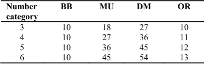
Table 4. The number of parameters used for different models by the number of different classes of response variables
Number
category BB MU DM OR
3 10 18 27 10
4 10 27 36 11
5 10 36 45 12
http://jbe.tums.ac.ir 69
Therefore, this discrete consideration of the response variable is negligible.
If we want to compare the models in terms of complexity and the number of parameters used in fitting the data, let's assume that the response variable has k classes and p independent variables (without consideration of the model constant), The beta-binomial, multinomial, dirichlet-multinomial and ordinal regression models estimate p + 2, (P + 1) * (k-1), (p + 1) * k and k-1 + p parameters during fit, respectively. In Table 4, the number of parameters that have been estimated for different models for the different number of classes of response variables are presented. Beta-binomial model with increase in number of classes for response
variables, the number of its parameters remains unchanged and does not depend on the number of classes. Ordinal regression model is also for an increase in number of classes, a parameter is added to the number of the ones need to be estimated. But the multinomial model, and specially the dirichlet-multinomial model, has a significant increase in the number of parameters due to increase in number of classes. In a given number of classes for response variables, the beta-binomial model uses a smaller number of parameters than other models; the ordinal regression model does not have lots of parameters, but the two models of multinomial regression, and especially the dirichlet-multinomial regression model, use a very high
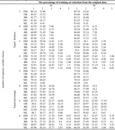
Table 5. Error percentage resulting from fitting of the models based on distance, considering different conditions The percentage of training set selection from the original data
30 50
1 2 3 4 5 1 2 3 4 5
number of
respo
nse variable clas
ses
Equal distance
3 DM 86.14 13.86 85.74 14.26
OR 84.47 15.53 85.04 14.96
BB 82.77 17.23 83.12 16.88
MU 81.83 18.17 82.55 17.45
ML 91.59 8.41 91.65 8.35
4 DM 62.95 31.09 5.96 61.92 31.75 6.33
OR 60.13 33.15 6.72 59.54 33.68 6.78
BB 60.89 31.45 7.66 60.48 32.14 7.38
MU 59.97 32.22 7.81 59.96 32.77 7.27
ML 85.96 12.4 1.64 86.85 11.53 1.62
5 DM 54.38 29.56 13.91 2.15 53.22 30.1 14.29 2.39 OR 53.12 29.2 15.42 2.26 52.15 29.46 15.91 2.48 BB 54.49 28.9 14.05 2.56 54.06 29.16 14.24 2.54
MU 54.17 28.5 14.24 3.09 52.6 29.58 14.94 2.88
ML 75.57 20.74 3.41 0.28 75.65 20.86 3.25 0.24 6 DM 53.18 25.55 15.02 5.24 1.01 52.02 26.07 15.65 5.2 1.06
OR 53.99 25.28 14.72 5.12 0.89 53.62 25.16 15.34 4.98 0.9 BB 52.8 25.71 15.15 5.26 1.08 52.46 25.52 15.9 5.07 1.05 MU 53.91 24.45 14.47 5.67 1.5 52.86 25.14 15.19 5.6 1.21 ML 70.61 22.74 5.39 1.22 0.04 71.32 22.51 4.96 1.2 0.01
Equal per
centag
e
3 DM 76.17 23.83 75.94 24.06
OR 81.69 18.31 82.73 17.27
BB 80.71 19.29 81.89 18.11
MU 79.35 20.65 79.53 20.47
ML 93.52 6.48 94.39 5.61
4 DM 43.53 38.19 18.28 42.28 38.42 19.3
OR 45.35 37.89 16.76 46.31 37.49 16.2
BB 40.63 37.05 22.32 39.06 37.69 23.25
MU 47.02 38.39 14.59 46.08 38.78 15.14
ML 64.23 33.95 1.82 64.93 33.53 1.54
5 DM 29.73 31.87 22.37 16.03 28.25 31.61 22.95 17.19 OR 30.8 29.27 23.56 16.37 30.27 28.97 23.92 16.84 BB 25.8 30.44 22.7 21.06 25.61 30.66 22.81 20.92 MU 33.09 33.23 21.05 12.63 31.61 32.94 21.73 13.72 ML 48.7 36.17 14.27 0.86 49.27 36.02 14.1 0.61 6 DM 37.37 27.37 21.54 9.05 4.67 36.42 26.7 22.47 9.23 5.18
number of parameters in comparison with the two previous models. While these two models, despite the use of a high number of parameters, had similar performances, and even lower than the beta-binomial and ordinal models. This is a very good feature for the beta-binomial model, even it uses the lowest number of parameter (compared to the comparative models in this study) it has the same performance, and in some cases a better one.
Now we compare the models based on their error. Suppose several models are the same in terms of error percentage in the response variable class, the issue is the severity of the error. Because here the variable is discrete and an ordinal type, the distance between the class
that is mistakenly predicted and the true class is important. For example, suppose that for a particular observation, the response variable is located on the second class, a model predicts first class and another predicts fifth class. Both models are in error. But the first model has less error than the second one. Based on the same 32 scenarios that we have considered, for different models their percentage of error were based on the distance between predicted class and the real class of the response variable are given in Table 5. For example, consider the dirichlet-multinomial model in the case where the percentage of the training set is 30%, the number of classes is 3, and the classification method were based on equal intervals. In this case,
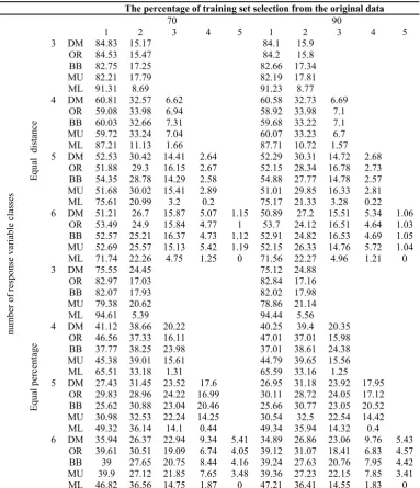
Table 5. Cntd
The percentage of training set selection from the original data
70 90
1 2 3 4 5 1 2 3 4 5
number of
respo
nse variable clas
ses
Equal distance
3 DM 84.83 15.17 84.1 15.9
OR 84.53 15.47 84.2 15.8
BB 82.75 17.25 82.66 17.34
MU 82.21 17.79 82.19 17.81
ML 91.31 8.69 91.23 8.77
4 DM 60.81 32.57 6.62 60.58 32.73 6.69
OR 59.08 33.98 6.94 58.92 33.98 7.1
BB 60.03 32.66 7.31 59.68 33.22 7.1
MU 59.72 33.24 7.04 60.07 33.23 6.7
ML 87.21 11.13 1.66 87.71 10.72 1.57
5 DM 52.53 30.42 14.41 2.64 52.29 30.31 14.72 2.68 OR 51.88 29.3 16.15 2.67 52.15 28.34 16.78 2.73 BB 54.35 28.78 14.29 2.58 54.88 27.77 14.78 2.57 MU 51.68 30.02 15.41 2.89 51.01 29.85 16.33 2.81
ML 75.61 20.99 3.2 0.2 75.17 21.33 3.28 0.22
6 DM 51.21 26.7 15.87 5.07 1.15 50.89 27.2 15.51 5.34 1.06 OR 53.49 24.9 15.84 4.77 1 53.7 24.12 16.51 4.64 1.03 BB 52.57 25.21 16.37 4.73 1.12 52.91 24.82 16.53 4.69 1.05 MU 52.69 25.57 15.13 5.42 1.19 52.15 26.33 14.76 5.72 1.04 ML 71.74 22.26 4.75 1.25 0 71.56 22.27 4.96 1.21 0
Equal per
centag
e
3 DM 75.55 24.45 75.12 24.88
OR 82.97 17.03 82.84 17.16
BB 82.07 17.93 82.02 17.98
MU 79.38 20.62 78.86 21.14
ML 94.61 5.39 94.44 5.56
4 DM 41.12 38.66 20.22 40.25 39.4 20.35
OR 46.56 37.33 16.11 47.01 37.01 15.98
BB 37.77 38.25 23.98 37.01 38.61 24.38
MU 45.38 39.01 15.61 44.79 39.65 15.56
ML 65.51 33.18 1.31 65.59 33.16 1.25
5 DM 27.43 31.45 23.52 17.6 26.95 31.18 23.92 17.95 OR 29.83 28.96 24.22 16.99 30.11 28.72 24.05 17.12 BB 25.62 30.88 23.04 20.46 25.66 30.77 23.05 20.52 MU 30.98 32.53 22.24 14.25 30.54 32.5 22.54 14.42 ML 49.32 36.14 14.1 0.44 49.34 35.94 14.32 0.4 6 DM 35.94 26.37 22.94 9.34 5.41 34.89 26.86 23.06 9.76 5.43
http://jbe.tums.ac.ir
71
86.14% of the errors are predicted with one class distance and 13.86% with two classes distance from the real one. Generally, in all models, the share of prediction error decreases with the increase in class distance between predicted and the real one. Therefore, the models have similar behaviors.
Conclusion
As stated before, the study was carried out in order to compare the power of fitting in beta-binomial model with other mentioned ones. We also implied that, in previous studies, the beta-binomial model in a number of ways, including high interpretability, simplicity of the model, the ability to identify the clinically influential variables, measuring the relationship between independent and dependent variables from a clinical point of view, has been found to be more appropriate. In this paper, we focused on the power of the models in fitting the quality of life data to compare the beta-binomial model with the other models. In addition to the good features of the beta-binomial in fitting, the model accuracy has been well-suited to fit in many different situations, and sometimes better than other models.
Acknowledgments
We thankful all people and friends who collaborated with us in this survey.
Conflict of Interests
In this study we have no conflict of interest.
References
1. Fayers PM, Machin D. Multi‐Item Scales. Quality of life: assessment, analysis and interpretation. John Wiley & Sons, Ltd; 2000:72-90.
2. Fayers PM, Machin D. Quality of life: the assessment, analysis and interpretation of patient-reported outcomes: John Wiley & Sons; 2013. 3. Mesbah M, Cole BF, Lee MLT. Statistical
methods for quality of life studies: design, measurements and analysis: Springer Science & Business Media; 2013.
4. Cox DR, Fitzpatrick R, Fletcher A, Gore S, Spiegelhalter D, Jones D. Quality-of-life assessment: can we keep it simple? J Royal Stat Soc Series A. 1992:353-93.
5. Walters SJ, Campbell MJ, Lall R. Design and analysis of trials with quality of life as an
outcome: a practical guide. J Biopharm Stat. 2001;11(3):155-76.
6. Arostegui I, Nunez-Anton V, Quintana JM. Analysis of the short form-36 (SF-36): the beta-binomial distribution approach. Stat Med. 2007;26(6):1318-42.
7. Madariaga IA, Antón VAN. Aspectos estadísticos del Cuestionario de Calidad de Vida relacionada con salud Short Form-36 (SF-36). Estadística española. 2008;50(167):147-92.
8. Arostegui I, Núñez-Anton V. Aspectos Estadísticos del Cuestionario de Calidad de Vida relacionada con la salud Short Form-36 (SF-36). Estadística española. 2008;50(167):147-92. 9. Arostegui I, Núñez-Antón V, editors. Alternative
modelling approaches for the SF-36 health questionnaire. Proceedings of the 22nd International Workshop on Statistical Modelling; 2007: Institut d’Estadística de Catalunya, Barcelona.
10. Arostegui I, Padierna A, Quintana JM. Assessment of HRQoL in patients with eating disorders by the beta‐binomial regression approach. Int J Eat Disord. 2010;43(5):455-63. 11. Arostegui I, Núñez-Antón V, Quintana JM.
Statistical approaches to analyse patient-reported outcomes as response variables: An application to health-related quality of life. Statistical methods in medical research. 2012;21(2):189-214.
12. Kaviani H, Seyfourian H, Sharifi V, Ebrahimkhani N. Reliability and validity of Anxiety and Depression Hospital Scales (HADS) &58; Iranian patients with anxiety and depression disorders. Tehran Uni Med J. 2009;67(5):379-85. 13. Montazeri A, Vahdaninia M, Mousavi SJ,
Omidvari S. The Iranian version of 12-item Short Form Health Survey (SF-12): factor structure, internal consistency and construct validity. BMC Pub Health. 2009;9:341.
14. Ihaka R, Gentleman R. R: a language for data analysis and graphics. J Comput Graph Stat. 1996;5(3):299-314.
15. Royston P, Altman DG, Sauerbrei W. Dichotomizing continuous predictors in multiple regression: a bad idea. Stat Med. 2006;25(1):127-41.
16. Altman DG, Lyman GH. Methodological challenges in the evaluation of prognostic factors in breast cancer. Prognostic variables in node-negative and node-positive breast cancer: Springer; 1998:379-93.