Allocation efficiency in network DEA

58

Available online at http://ijdea.srbiau.ac.ir Int. J. Data Envelopment Analysis (ISSN 2345-458X)

Vol. 1, No. 2, Year 2013 Article ID IJDEA-00124, 12 pages Research Article

Allocation efficiency in network DEA

S. Banihashemi

*a

, G.Tohidi

b

(a) Department of mathematics, Computer and Statistics, Allame Tabataba’i University, Tehran, Iran. (b) Department of Mathematics, Islamic Azad University, Central Tehran Branch, Tehran-Iran.

Abstract

The present study is an attempt towards remodeling cost, revenue and profit relationship within the network process. The previous models of Data Envelopment Analysis (DEA) have been too general in their scope and focused on the input and the output within a black box system, therefore they have not been able to measure various phases simultaneously within a network system. By using these models internal linking activities are neglected. A slacks-based network DEA model is dealt with intermediate products (Tone,Tsutsui). In this development, each input and output can use situations where unit price and unit cost information are available. In this paper we introduce models of cost, revenue and profit efficiency in network DEA. These models are illustrated by numerical examples and finally results of Constant Returns to Scale (CRS) are obtained. The findings could be used in minimizing the costs and maximizing the benefits in various organizations, public services, factories, and public and private sector companies.

Keywords: Data Envelopment Analysis (DEA), New Network Cost Efficiency (NNCE), New Network Revenue Efficiency (NNRE), New Network Profit Efficiency (NNPE).

1 Introduction

Network DEA models were introduced in the innovative book [4] by Fare and Grosskopf. They investigated the so-called “black box” for the first time. Their models were extended by several authors. The network DEA model [6] proposed by Lewis and Sexton has a multi-stage structure as an extension of the two-stage DEA model proposed in Sexton and Lewis [10]. This study solves a DEA model for each node independently. For an output-oriented model, firstly a general DEA model is solved for the upstream node at the 1stage to obtain the optimal solution of outputs. At the next stage, a part of (or all of) optimal outputs obtained at the upstream node are applied as intermediate inputs to the next node. After solving DEA models for all nodes in turn, a final optimal output is obtained at the last node. The firm-level efficiency score is measured as the final optimal output divided by an

* _{Corresponding author, email address: [email protected]. Tel:+98 21 22494938.}

observed output. Prieto and Zofio [8] applied network efficiency analysis within an input-output model initiated by Koopmans [5]. They optimized primary input allocations, intermediate products and final demand products by way of network DEA techniques. Lothgren and Tambour [7] applied network DEA model to a sample of Swedish pharmacies. The above network DEA models utilize the radial measure of efficiency, e.g. the CCR (Charnes et al. [2] or the BCC (Banker et al. [1].In 2008, Tone and Tsutsui [11] published a network DEA model but uses the slacks-based measure (SBM is a non-radial method). This paper introduces a network DEA model (by uses the slacks-based measure) that each input and output and linking activities have unit price and unit cost information.

In the next section Technical efficiency, Cost efficiency and Network DEA (NDEA) models based on the weighted slacks-based measure (WSBM) are proposed .Then in section 3 we introduced New Network Cost Efficiency (NNCE), New Network Revenue Efficiency (NNRE), New Network Profit Efficiency (NNPE). Illustrative examples are introduced in section 4. And finally the results the paper in the last section summarized.

2 Background

Data envelopment analysis (DEA) is a non-parametric method that uses mathematical programming techniques to evaluate the performance or relative efficiency of Decision Making Units (DMUs); e.g., teams, people, branches of banks, hospitals, schools, etc., in terms of multiple inputs and outputs. Originally developed by Charnes et al. (1978), the techniques have been further developed and expanded to a wide variety of applications in different contexts including education, health care, banking, education, armed forces, market research, manufacturing, etc. (Charnes et al. 1994). Not only are the DEA models used to evaluate efficiency, but also to compare each DMU to the best production units possible. According to Fare, Grosskopf, & Lovell (1994), the PPS (Production Possibility Set) is defined as the set of all inputs and outputs of a system in which inputs can produce outputs. DEA models can be input-oriented and output -oriented. Likewise, DEA models can address constant returns to scale (CRS) and variable returns to scale (VRS). One of the drawbacks of these models is the neglect of internal or linking activities. For example, many companies are comprised of several divisions that are linked as illustrated in numerical example. In the example the company has three divisions. Each division utilizes its own input resources for producing its own outputs. However, there are linking activities as shown by link 1→ 2, link 1 → 3 and link 2→ 3. Link 1→ 2 indicates that part of the outputs from Division 1 are utilized as inputs to Division 2. In traditional DEA models, every activity should belong to either an input or an output but not to both. Thus, these models cannot deal with intermediate products formally. DEA models also can calculate technical efficiency and can evaluate types of inefficiency such as cost efficiency, revenue efficiency and profit efficiency when information on prices and costs are available.

2.1 Technical efficiency

Technical efficiency depicts the capability of production units to transform inputs into outputs. Consider 𝐷𝑀𝑈_𝑗(j=1,…, n) where each DMU consumes m inputs to produce s outputs. Suppose that the observed input and output vectors of𝐷𝑀𝑈_𝑗be

𝑌_𝑗≥ 0, 𝑌_𝑗≠ 0.

In continue, the Production Possibility Set T_cis defined as:

𝑇_𝑐= {(𝑋, 𝑌)|𝑋 ≥ ∑ 𝜆_𝑗𝑋_𝑗

𝑛

𝑗=1

, 𝑌 ≤ ∑ 𝜆_𝑗𝑌_𝑗

𝑛

𝑗=1

, 𝜆_𝑗 ≥ 0, 𝑗 = 1, … , 𝑛}

By the production possibility set above, the CCR model that used to evaluate technical efficiency as follows:

𝑇𝐸_𝑜= 𝑀𝑖𝑛 𝜃_𝑜

S t. ∑𝑛_𝑗=1𝜆_𝑗𝑥_𝑖𝑗 ≤ 𝜃_𝑜𝑥_𝑖𝑜 i=1,…, m,

∑𝑛_𝑗=1𝜆_𝑗𝑦_𝑟𝑗≥ 𝑦_𝑟𝑜 r=1,…, s, 2.1

𝜆_𝑗 ≥ 0 j=1,…,n,

𝜃free.

The CCR assumes “constant returns to scale (CRS)” based on which increasing the investment by one unit generates the output only by one unit. The CRS assumption is appropriate when all DMUs operate at an optimal scale. However, government regulations, constraints on finance and so on, may cause a DMU not to operate at optimal scale. The use of the CRS specification when not all DMUs are operating at the optimal scale, results in measures of technical efficiency (TE) that are confounded by scale efficiencies. In another model of DEA, the BCC model assumes “variable returns to scale”, that is, the scale of output is varying. The use of the VRS specification permits the calculation of TE devoid of these scale efficiency effects. The CRS can be easily modified to account for VRS by adding the convexity constraint: ∑𝑛_𝑗=1𝜆_𝑗= 1. The efficiency value calculated in CCR is the “overall technical efficiency”, whereas the efficiency value computed by BCC is “pure technical efficiency” (PTE). The former divided by the latter is “scale efficiency” (SE). It must be noted that TE and PTE are greater than zero and less or equal to one (Rayeni &Saljooghi,[9] 2012).

Traditional DEA models deal with measurements of relative efficiency of DMUs regarding multiple-inputs and multiple outputs .Via employing these models, internal linking activities are neglected. Unlike such models, Network DEA model deals with intermediate products (Tone & Tsutsui, 2009).

2.2 Cost efficiency

Cost efficiency is defined as the effective choice of inputs vis a vis prices with aimed to minimize production costs, whereas technical efficiency investigates how well the production process converts inputs into outputs. It should be noted that DEA can also be used to measure cost efficiency (Rayeni & Saljooghi [9] (2012).

Considering this when input costs are available, there are two different situations: one common unit prices and costs for all DMUs and the other with different prices and costs from DMU to DMU. In this paper, different costs and prices are considered from DMU to DMU. Again, consider n decision making units (DMUs) with m inputs for producing s outputs. For𝐷𝑀𝑈𝑗, an input–output bundle

(𝑋 = (𝑥₁, 𝑥₂, … , 𝑥_𝑛) ∈ 𝑅𝑚×𝑛 _{, 𝑌 = (𝑦}

which the inputs have costs 𝐶 = (𝑐₁, 𝑐₂ , … , 𝑐_𝑛).

Let us define another cost-based production possibility set 𝑃_𝑐as:

𝑃_𝑐 = {(𝑥̅ ≥ 𝑋̅𝜆, 𝑦 ≤ 𝑌𝜆, 𝜆 ≥ 0}

Where 𝑋̅ = (𝑥̅₁, … , 𝑥̅_𝑛)𝑤𝑖𝑡ℎ𝑥̅_𝑗 = (𝑐_1𝑗𝑥_1𝑗, … , 𝑐_𝑚𝑗𝑥_𝑚𝑗). In order to obtain a measure of cost efficiency, when the input and output data are known and the prices differ from DMU to DMU, minimal cost model proposed by (Cooper, Seiford, &Tone, 2006[9]) could be used as follows:

𝑒𝑥̅∗= Min 𝑒𝑥̅

S t. 𝑥̅ ≥ 𝑋̅𝜆, 2.2

𝑦_𝑜 ≤ 𝑌𝜆,

𝜆 ≥ 0

The CE measure is given by the ratio of the minimal cost value obtained from the above model to the current cost at𝐷𝑀𝑈_𝑜 as follows:

Cost Efficiency = 𝛼∗ = 𝑒𝑥̅_𝑜∗ / e𝑥̅_𝑜

In technology efficiency we focused on the network DEA where unit price and unit cost information are not available .Technology and cost are the wheels that drive modern enterprises, hence the management is eager to know how and to what extent their resources are being effectively and efficiently utilized, compared to other similar enterprises in the same or a similar field. Regarding this subject, there are two different situations: one with common unit prices and unit costs for all DMUs and the other with different prices and costs for all DMUs. So we introduce new network cost efficiency along with new network revenue efficiency and new network profit efficiency.

2.3 Network DEA based on slacks-based measure (NSBM)

n DMUs ((𝑗 = 1, … , 𝑛) consist of 𝑘 divisions (𝑘 = 1, … , 𝑛) exist. Let m_kand r_kbe the numbers of inputs and outputs to division𝑘. Link leading from division 𝑘 to division ℎ represented by (𝑘, ℎ) and set of links by 𝐿. The observed data are { 𝑥_𝑗𝑘 ∈ 𝑅₊𝑚𝑘 _{} ( 𝑗 = 1, … , 𝑛 ∶ 𝑘 = 1, … , 𝑘), {𝑦}

𝑗𝑘 ∈ 𝑅−𝑟𝑘} (𝑗 =

1, … , 𝑛 , 𝑘 = 1, … , 𝑘) and {𝑧_𝑗(𝑘,ℎ)∈ 𝑅₊𝑡(𝑘,ℎ)} (𝑗 = 1, … , 𝑛, (𝑘, ℎ) ∈ 𝐿) .

The production Possibility Set (PPS) is defined by

( , ) ( , ) ( , ) ( , ) ( , )

{( , , ) | , , ( ), ( ),

1, 0}

k k k h k k k k k k k h k h k k h k h h k

P x y z x X y Y z z as outputs k z z as inputs h

e

   

 

    

 

Suppose that below model (input oriented efficiency 𝜃_𝑜 )have variable returns to scale (VRS) and

(NSBM) 𝜃_𝑜= Min ∑𝐾 𝑤𝑘 𝑘=1

[1-1 𝑚_𝑘(∑

𝑠𝑖𝑘−

𝑥_𝑖𝑜𝑘 𝑚𝑘

𝑖=1 )]

( , ) ( , )

( , ) ( , )

( , ) ( , )

( , ) ( , )

1 .

( 1,..., ),

( 1,..., ),

1 ( 1,..., ),

0, 0, 0 ( 1,..., ),

( ( , )), ( )

( ( , ))

, ( ( , )), ( )

(

k k k k o

k k k k o

k

k k

k

k h k h h o

k h k h k o

k h h k h k

k h k h s t

x x s k K

y y s k K

e k K

s s k K

Z Z k h a

Z Z k h

or

Z Z k h b

where

Z Z

















 

 

  

  

 

   

 

 

 

 ( , ) ( , )

,..., k h ) tk h n

n

Z R 

2.3

Where

𝑋𝑘_=(𝑥

1𝑘, … , 𝑥𝑛 𝑘) ∈ 𝑅𝑚𝑘×𝑛

𝑌𝑘= (𝑦₁𝑘,…,𝑦𝑛𝑘) ∈ 𝑅𝑟𝑘×𝑛

And 𝑠𝑘−_(𝑠𝑘+_{) are the input (output) slack vectors.}

(a) The “free” link value case.

The linking activities are freely determined (discretionary) while keeping continuity between input and output.

(b)The “fixed” link value case.

The linking activities are kept unchanged (non- discretionary)

3 Allocation efficiency

3.1 New Network Cost Efficiency (NNCE)

( , ) _{( , ) ( , )} ( , ) ( , )

1 1 _{1 1}

( , ) ( , ) ( , ) ( , )

( , )

1 _{1 1}

{( , , ) | , , ( ), ( ),

1, 0}

( ,..., ), ( ,..., )

( ,..., ), ( ,...,

k

k _k k h k k _{k k k k k h k h k} k h k h _h c

k

k k k

k k k k j j j mj mj k h k h k h k h

k k h n j _{j j}

P x y z x X y Y z z as outputs k z z as inputs h

e

x x x x c x c x

z z z z c z

                  ( , ) )

k k h mj mj

c z

Based on this new Production Possibility, Set 𝑃_𝑐 ,



*k , is obtained as the following LP problem:

NNCE=

*

*( , )

1

k

K _{k h}

h o k o x z   





( , ) 1 ( , ) ( , ) ( , ) ( , ) ( , ) _{( , )} Min

: 1,..., ,

1,..., ,

, ( ( , )), ( ) 3.1

, ( ( , )), , ( ( , )), ( ) 1, 0, 0 k K k h k h

k k _k

k k k o

k h k h _h o

k h k h k o

k h _{h k h k}

k k h

x z

st x X k K

y Y k K

z z k h a

z z k h

or

z z k h b

e



















              





The New Network Cost Efficiency is defined as:

* *( , )

* ( , )

1 1 1

( ) / ( )

k k h k

K K K

k k h

o o o o

k k k h

x z x z



  















Where 𝑒 ∈ 𝑅𝑚 _{is a row vector with all elements being equal to 1.}

3.2 New Network Revenue Efficiency (NNRE)

In this section we deal New Network Revenue Efficiency (NNRE) on Network Slack Based Measure (NSBM) that prices play a role in the PPS on output (consists of output and output from k):

( , ) ( , ) ( , ) _{( , ) ( , )}

1 1 1

( , ) ( , ) ( , ) ( , ) _{( , )}

1 _{1 1}

{( , , ) | , , ( ), ( ),

1, 0}

( ,..., ), ( ,..., )

( ,... , ), ( ,...,

k k k

k k h k k k h k h

k k k k k k k h k h h p

k

k _{k k k k} n j j j mj mj k h k h k h k h _{k k h}

n j _{j j}

P x y z x X y Y z z as output k z z as input h

e

y y y y p y p y

z z z z p z

                    ( , ) )

k k h rj rj

p z

Based on this new Production Possibility, Set 𝑃_𝑝 ,



*k, is obtained as the following LP problem:

NNRE=

*

*( , )

1

k

K _{k h}

o o k k y z   





( , ) 1 ( , ) ( , ) ( , ) ( , ) ( , ) _{( , )} Max : 1,..., 1,..., , ( ( , ))

, ( ( , )) ( ) 3.2

, ( ( , )) ( )

1

0, 0

k

K _{k h}

k k

k k k o

k k _k k h k h _k o

k h k h h o

k h _{k k h h} k

k h

y z

st x X k K

y Y k K

z z k h

z z k h a

or

z z k h b

e



















              





The New Network Revenue Efficiency, is defined as:

* * ( , ) *( , ) 1 1 ( ) / ( ) k k K K

k k h k h

o o o o

k k k k

y z y z





 















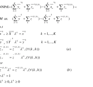
3.3 New Network Profit Efficiency (NNPrE)

NNPrE= * * *( , ) *( , ) 1 1 ( ) ( ) k k

K _{k h} K _{k h}

o o o o

k k k h

y z x z

    









= ( , ) ( , ) 1 1 ( , ) ( , ) ( , ) ( , ) ( , ) ( , )

ax ( ) ( )

.

1,...,

1,...,

, ( ( , )) ( ) 3.3

, ( ( , ))

, ( ( , )) ( )

1

0, 0

k k

k _{k h} K _{k h}

k k k h

k k _k k o

k

k _k k o

k h k h _k o

k h k h h o

k h _k k h _h

k k h

M y z x z

s t

x X x k K

y Y y k K

z z k h a

z z k h

or

z z k h b

e



















                      









Here, the purpose is to find a profit-maximization in the Production Possibility Set (PPS):

( , ) ( , ) ( , ) ( , ) ( , )

{( , , , ) | , , ( ), ( ),

1, 0}

k k k h k k _k k k _k k h k h _k k h k h _h pc

k

P x y z x X y Y z z as output k z z as input h

e

   

 

    

 

Based on an optimal solution, the New Network Profit Efficiency can be defined in ratio form by:

* *

* _{( , ) ( , ) *( , ) *( , )}

1 1 1 1

{( ) ( )} / {( ) ( )}

k _K k _K k _K k _K k

k h k h k h k h

o o o o o o o

k k k h k k k h o

y z x z y z x z





   































4 Numerical example

A numerical example by ten DMUs is represented for obtaining New Network Cost Efficiency (NNCE) and New Network Revenue Efficiency (NNRE). A list of data is provided in Table 1. Table 1 consists of inputs, unit input cost, outputs, unit output price in three divisions. Unit input link cost, unit output link price are shown in Table 2.



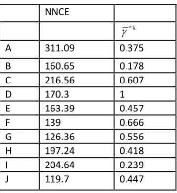
*kis obtained by using model 3.1. results are shown in Table 3. DMU_Dis cost efficient. In Table 4 cost efficiency is calculated for each division separately.

*k

Table 1

Consists of inputs, unit input cost, outputs, unit output price in three divisions.

Div1 Div2 Div3

DMU Input1 C1 Input2 C2 Output2 P2 Input3 C3 Output3 P3

A 0.838 250 0.277 120 0.879 900 0.962 220 0.337 687

B 1.233 500 0.132 180 0.538 739 0.443 210 0.18 194

C 0.321 125 0.045 290 0.911 142 0.482 140 0.198 285

D 1.483 113 0.111 60 0.57 863 0.467 150 0.491 401

E 1.592 50 0.208 85 1.086 307 1.073 200 0.372 179

F 0.79 45 0.139 95 0.722 1200 0.545 85 0.253 1054

G 0.451 95 0.075 100 0.509 270 0.366 150 0.241 394

H 0.408 450 0.074 140 0.619 987 0.229 230 0.097 276

I 1.864 200 0.061 130 1.023 356 0.691 160 0.38 840

J 1.222 10 0.149 45 0.769 470 0.337 450 0.178 161

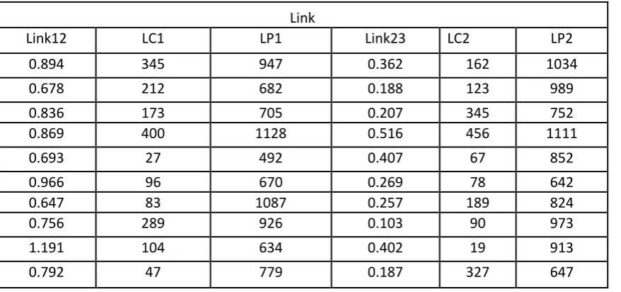
Table2

Unit input link cost, unit output link price are shown.

Link

Link12 LC1 LP1 Link23 LC2 LP2

0.894 345 947 0.362 162 1034

0.678 212 682 0.188 123 989

0.836 173 705 0.207 345 752

0.869 400 1128 0.516 456 1111

0.693 27 492 0.407 67 852

0.966 96 670 0.269 78 642

0.647 83 1087 0.257 189 824

0.756 289 926 0.103 90 973

1.191 104 634 0.402 19 913

0.792 47 779 0.187 327 647

*k

Table3

NNCE

*k



A 311.09 0.375

B 160.65 0.178

C 216.56 0.607

D 170.3 1

E 163.39 0.457

F 139 0.666

G 126.36 0.556

H 197.24 0.418

I 204.64 0.239

J 119.7 0.447

Table 4

Cost efficiency is calculated for each division separately.

A 103.77 44.42 89.51 0.495 0.127 0.331 0.954

B 47.13 21.94 47.81 0.076 0.131 0.412 0.619

C 47.42 50.42 52.59 0.789 0.32 0.379 1.488

D 114 165.14 130.42 0.681 0.466 0.425 1.572

E 6.13 36.3 98.81 0.077 1 0.409 1.486

F 30.4 25.29 67.2 0.856 0.239 1 2.095

G 17.61 34.05 64.01 0.28 0.556 0.619 1.456

H 71.63 20.69 25.76 0.39 0.091 0.417 0.898

I 40.6 34.19 100.93 0.109 0.093 0.855 1.057

J 12.2 42.9 47.28 1 1 0.222 2.222

*k

Table5

NNRE

*k



A 1046.51 0.648

B 3254.68 0.331

C 1364.43 0.682

D 4051.34 0.553

E 4127.62 0.263

F 2755.9 0.709

G 1774.38 0.647

H 1621.82 0.885

I 4491.12 0.402

J 3414.86 0.33

5 Conclusion

In this paper have been proposed cost, revenue and profit efficiency in network DEA by variable cost and variable price for inputs, outputs and links any divisions. All models considered with constant returns to scale (CRS). We represented by using numerical example that under the variable returns to scale (VRS) assumption (if we used common unit input price) models are infeasible

Reference

[1]Banker.R.D, Charnes .A, Coopper .W.W, Some models for estimating technicaland scale inefficiencies in data envelopment analysis, Management Science30 (9) (1984) 1078_1092.

[2] Charnes A,Cooper WW, RhodesE(1978).Measuring the efficiency of decision making units. European Journal of Operational Research 2(6), 429-444.

[3] Cooper, Seiford and Kaoru Tone.Data Envelopment Analysis and its uses.

[4] Fare R,Grosskopf S(1996) Intertemporal Production Frontiers: With Dynamic DEA.Kluwer Academic Publishers,Boston.

[5] Koopmans T (1951) An analysis of production as an efficient combination of activities.In Activity analysis of production and allocation. In Koopmans T (Ed.) Cowles commission for research in economics, monograh, 13, John Wiley and Sons, New York.

[6] Lewis HF, Sexton TR (2004) Network DEA: efficiency analysis of organization with complex internal structure, Computers & Operations Research 31, 1365-1410.

[8] Prieto AM, Zofio JL (2007) Network DEA efficiency in input-output models: With an application to OECD countries, Europan Jornal of Operational Research, 178, 292-304.

[9] Rayeni,MM,Saljooghi.F(2012).Equitable allocation of fixed costs and its effect on technical and cost efficiency: Case study in universities.Afr.J.Business Management.1263-1269

[10]Sexton TR, Lewis HF (2003) Two-stage DEA: An application to major league baseball, Jornal of Productivity Analysis, 19, 227-249.