Vol. 48, No. 2, Fall 2016, pp. 101-111
Please cite this article using:
Davari, N., Gholami, A., and Shabani, M., 2016. “Performance Enhancement of GPS/INS Integrated Navigation System Using Wavelet Based De-Noising Method”. Amirkabir International Journal of Electrical and Electronics Engineering, 48(2), pp. 101–111.
DOI: 10.22060/eej.2016.824
URL: http://eej.aut.ac.ir/article_821.html
*Corresponding Author, Email: [email protected]
Performance Enhancement of GPS/INS Integrated
Navigation System Using Wavelet Based De-Noising Method
N. Davari1,*, A. Gholami2, M. Shabani3
1- Ph.D. Student, Department of Electrical and Computer Engineering, Isfahan University of Technology, Isfahan, 84156-83111, Iran 2- Associate Professor, Department of Electrical and Computer Engineering, Isfahan University of Technology, Isfahan, 84156-83111, Iran
3- M.Sc., Department of Electrical and Computer Engineering, Isfahan University of Technology, Isfahan, 84156-83111, Iran
(Received 3 July 2015, Accepted 31 July 2016)
The accuracy of Inertial Navigation System (INS) is limited mainly by inertial sensors imperfections. Before using inertial signals in the datafusion algorithm, noise removal procedure should be done. In order to remove the noise, wavelet decomposition method is used in which the raw data are decomposed into high and low-frequency data sets. In this study, wavelet multi-level of decomposition technique is
used as an efficient pre-filter method for inertial measurements to improve the performance of INS. This
technique improves navigation accuracy by eliminating the high-frequency noise of inertial measure-ments. Optimum values of the level of decomposition are selected to obtain minimum error. Success-fully performing the de-noising process improves the sensors’ signal-to-noise ratios and removes short
term errors mixed with motion dynamics and finally provides cleaner and more reliable data to the INS. In this paper, the performance of an error state Kalman filter based GPS/INS integrated navigation sys -tem is studied using real measurement during GPS outages. The GPS/INS integrated navigation sys-tem used in this work is the loosely coupled structure. Results show that the average value of the root mean square of the position errors (as a measure of the quality of de-noising) during GPS outages using the WMRA procedureis reduced about 14% compared to those using the raw inertial measurements.
KEYWORDS:
GPS/INS Integrated Navigation, GPS Outages, Wavelet Analysis, Error State Kalman Filter, Level of Decomposition
1- Introduction
Most navigation systems use inertial sensors (accelerometers and gyroscopes). An inertial navigation system (INS) has a good accuracy in a short time, but the error grows with the elapse of time without bounds, while GPS has a high accuracy in a long time. Thus, INS and GPS integration could improve navigation accuracy for all times [1].
Conventional Kalman filtering (KF) [2] has been
the widely the implemented and accepted procedure for integrating the inertial navigation systems (INS)
with auxiliary sensors. The Kalman filter has been
implemented in two approaches, total state space and error state space methods, which are named direct and
indirect filtering, respectively [3,4]. In recent years, the indirect filtering is used mostly in the integrated
navigation systems [5,6]. Some literature reported
the direct filtering based integrated navigation system
[7-9]. In the case of GPS outages (signal blockages), the INS positioning error will increase in time until the GPS signals are available again. As soon as the GPS signals become available, it provides position information that may lead to compensation of INS errors [10].
The primary concern when working with a low-performance inertial measurement unit (IMU) is that the navigation solution degrades rapidly in the absence of an aiding source (which is mainly GPS). However, the navigation is still facing problem in places where the GPS signal gets lost, that commonly occur in urban areas and in unsuitable weather condition. In the case of GPS outages, the INS is used alone for positioning until the GPS signals are available again. One of the major issues that limits the INS accuracy, as a stand-alone navigation system, is the level of sensor imperfections especially its noise [11].
The noise affecting inertial sensors contains two parts: a low-frequency and a high-frequency component. Both components are combined together and affect the inertial sensor accuracy. The high-frequency component has white noise characteristics, while the low-frequency component (more commonly termed bias drift) is characterized by correlated noise. One way to deal with high-frequency noise is to de-noise the inertial sensor measurements prior to processing. In this study we can remove the effect of the short-term error of the stand-alone INS only, while the long-term error can often be modeled
with sufficient accuracy as a stochastic process, and
be estimated and compensated using data fusion
techniques like Kalman filter [12].
In order to enhance the final accuracy of the
system especially during GPS outages, it is necessary
to use an appropriate pre-filtering method to the raw IMU data. Applying efficient pre-filter successfully
improves the sensors signal-to-noise ratios, removes short-term errors mixed with motion dynamics, and provides more reliable data. Conventional de-noising methods include moving average and
low-pass filtering techniques. In recent years, wavelet
decomposition is more often presented as an effective method to cope with the inertial sensor noise. Several other novel methods, such as neural network de-noising [13] have also been widely investigated. The wavelet enormous advantages compared with other methods of signal processing are summarized by Sifuzzaman et al. [14]. In these methods, preventing
over-smoothing effects is too difficult, because
there is no rigorous criterion to evaluate the cut-off frequency or the wavelet de-noising levels [15].
The wavelet transform (WT) is a powerful tool for signal and image processing. From the mid-1980s, it has been successfully used in many
scientific fields such as signal processing, image
compression, computer graphics, pattern recognition and de-noising of medical imaging [16]. One way to remove high frequency noise of the inertial sensor signals is to use wavelet technique prior to processing. Wavelet decomposition is a process in which a signal is successively broken down into low and high-frequency components [12,17]. Several studies have focused on evaluating the advantages of this technique, for instance, Nassar [17], Chiang et al. [10], and Abdel-Hamid et al. [18]. Skaloud [12] used wavelet decomposition technique for de-noising
of INS data and achieved a significant reduction
in estimated attitude errors. Bruton et al. [19] used WMRA to improve the estimation of airborne gravity disturbance values. Zhang et al. [20] also introduced a model using wavelet multi-resolution analysis and neural network to assist KF when GPS outages happen. The trained neural network can be employed to remove high-frequency noise and improve system accuracy. Noureldin et al. [21] integrated
neuron-wavelet algorithm and Kalman filter to de-noising and
fused the outputs of INS/GPS and provided precise positioning information for the vehicle.
drift of 1.0–10.0 deg/h and accelerometer bias of 1-5
mg) in order tominimize the undesirable effects of sensor noise and other high-frequency disturbances. In Sect. 4, we show that the position errors obtained from de-noised INS data will be smaller than the ones obtained from the original data.
This paper is organized as follows: Section 2 describes the basic information of the Wavelet transform (WT) and the principle of wavelet multi-resolution analysis. Section 3 presents wavelet de-noising method implemented to the INS/GPS integrated navigation system. It contains the structure
of INS/GPS integrated system and Kalman filter used
in the integration of the system. The experimental results and the effect of de-noising INS data in INS/ GPS integration with some simulated GPS outages are analyzed in section 4. Finally, the conclusion is given in section 5.
2- Wavelet de-noising technique
2- 1- Discrete wavelet transform (DWT)Wavelet transform is able to eliminate noise and compression of signals without the original signal deterioration. The wavelet transformation of a
time-domain signal is defined in terms of the projections
of this signal into a family of functions that are all normalized dilations and translations of wavelet functions [22]. Wavelet techniques are based on analyzing a signal through signal windowing but with variable window sizes. The major advantage of wavelets transform relative to other signal processing techniques is a capability to analyze a localized portion of a large signal [23]. This is possible since wavelet transform applies the wide window (long time intervals) to analyze a low-frequency component of the signal and the narrow window (short time intervals) to analyze a high-frequency component of the signal [24].
The low frequency fraction of the IMU sensor data is the signal of interest (motion dynamics) and the high frequency component is usually the signal noise. In the implementation of the DWT, the wavelet
coefficients of a signal are computed by passing
such a signal through two complementary half-band
filters, the output of the low-pass filter (LPF) is called
approximation part while the output of high-pass
filter (HPF) is called details part (see Fig. 1). For
more details on the design of decomposition and corresponding reconstruction LPF and HPF, see [25]. A good review of statistical properties of wavelet
coefficients can be found in [26] and [27].
Since we are dealing with discrete-time inertial sensor signals, the DWT is implemented. The wavelet
coefficients of a discrete time sequence, x(n), is given as [25,28]:
(1)
(2) where aj,k and dj,k are the approximation coefficient and the details coefficient at the j-th resolution level, respectively, Φj,k(n) is the scale function, Ψj,k(n) is the wavelet function and 2-j/2Φ(2-jn-k), 2-j/2Ψ(2-jn-k)
are the scaled and shifted versions of Φj,k(n) and
Ψj,k(n) respectively, based on the values of j (scaling
coefficient) and k (shifting coefficient). The original
signal x(n) can be generated from the corresponding wavelet function using the following equation:
(3) The wavelet function should be short and oscillatory; in other words, it should have zero average and decay quickly at both ends. This condition ensures that the summation in the DWT equation is
finite [29,30].
2- 2- Signal de-noising using Wavelet multi-level of decomposition
The wavelet multi-resolution analysis or wavelet multiple Level of Decomposition (LOD) is a procedure in which a signal is broken down into various resolution levels [12,23]. Therefore,
to obtain finer resolution frequency components Fig. 1. Signal Decomposition by the Discrete Wavelet
of a specific signal, the signal is broken down into
many lower-resolution components by repeating the DWT decomposition procedure with successive decompositions of the obtained approximation parts (see Fig. 2). Using wavelet multi-resolution analysis,
the signal can be represented by a finite sum of
components at different resolutions and hence, each component can be processed adaptively depending on the application at hand [23]. Applying WMRA to
the inertial signal comprises two main steps. The first
involves eliminating the high-frequency sensor noise using wavelet de-noising methods. The second step then follows by specifying a proper threshold through which the motion dynamics can be separated from the short-term and/or long-term sensor errors as well as other disturbances.The approximation part includes the long term noises, the earth gravity and rotation rate frequency and dynamic of vehicle motion. The WMRA is unable to separate long-term noise and the IMU readings. Thus, it must be removed by the appropriate integration algorithm using auxiliary sensors. The details part includes the undesired high-frequency noise components of the IMU and a lot of noise disturbances such as vehicle vibration.
The WMRA algorithm is presented in four main stages to remove noise from the data:
1) Choosing anappropriate value for LOD is very important. The selection is based on the removal high-frequency noise while keeping all the useful information in the signal. LOD selection criteria for static and kinematic mode data have been further reviewed in [31]. To select an appropriate LOD for static inertial data, several decomposition levels are applied and the standard deviation (STD) value of the high frequency component can be calculated for each
Fig. 2. Wavelet multi-resolution analysis (considering three levels of decomposition) [12]
obtained approximation component. The acceptable LOD will be the one after which the STD reaches its minimum value. To select an appropriate LOD for kinematic inertial data, in the beginning, a spectral analysis of the kinematic INS sensor raw data should be performed to ensure that the de-noising process does not remove any actual motion information. The vehicle motion dynamics is usually in the low-frequency portion of the spectrum. Then, by analyzing the spectrum, the frequency range of dynamic motion is detected. Therefore, the appropriate LOD can be selected to remove only the components that have frequencies higher than the detected motion frequency range.
2) Selection of the appropriate wavelet function.
The wavelet transform has various types of filters such as Daubechies, Coiflet, Biorsplines and Symlets which have different coefficients. To achieve optimal
performance in de-noising and minimize RMSE in navigation, one needs to choose an appropriate wavelet function.
3) Then, in order to reject the noise, a threshold
is set for the obtained detail coefficients at each level. Setting a threshold can be classified into hard and soft
thresholding as described by Burrus et al. [22]. The choice of the threshold value is crucial to the quality of the de-noising process. Several different methods were offered to calculate the amount of threshold by Ma et al. [32], Li and Zhao [33], Veterli et al. [34] and Misite et al. [35].
4) Reconstruct the de-noised signal using the linear combination of the details and approximation
coefficients which have been obtained at each level.
Then, the inverse wavelet transform is applied to this de-noised signal.
3- INS-GPS integrated navigation system
us-ing wavelet-based de-noisus-ing method
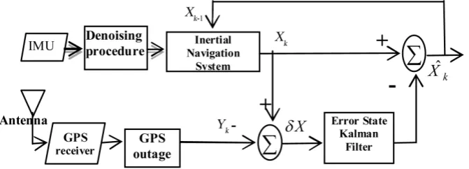
The structure of the INS/GPS integration system used in this study is shown in Fig. 3. The state variables, Xk, of the error state Kalman filter
consist of position error, velocity error, attitude error, accelerometer bias, and gyro bias. The measurement vector, Yk, of the Kalman filter is the position error
between the states and the new measurement of GPS. Inertial sensor signal after the noise removal process has been used for INS.
Fig. 3. IMU/GPS integrated navigation system structure
and accelerometers and the appropriate LOD of each signal is acquired. The wavelet transform is
applied to calculate the coefficients and then, the
inverse wavelet transform is used to reconstruct the decomposed signal. The de-noised signal is used to execute the INS/GPS integrated navigation. The
process is described briefly in the flowchart shown
in Fig. 4.
The following, firstly, the equations related to the
position, velocity, orientation and bias in an SDINS
are briefly reviewed. In the following, the system and
measurement error states equations for navigation and procedure of the KF are described.
3- 1- The SDINS
The acceleration and angular rate measurement vectors of the accelerometer and gyroscope f ̃b and ω̃b
ib
respectively, are modeled by:
(4) (5)
where b and q are bias and measurement noise,
respectively. The acceleration and angular rate vectors are corrected as follows:
(6) (7)
Fig. 4. Flowchart of the De-noising procedure
The accelerometer and gyro bias are modeled as random walks plus random constants, where:
(8)
(9) where baC and bgC are random constants, ωba and ωbg
are driving noise vectors assumed to be Gaussian white noise with zero mean and known variances, σba2
and σbg2, respectively.
The system state vector, x, consists of position, velocity, attitude, and bias. The vector is estimated by numerical integrationof the IMU measurements and dynamic equations of the system.
(10) where L̂, l̂ and d̂ are latitude, longitude, depth, and
v̂N, v̂E and v̂D are east velocity, north velocity, down velocity and Φ̂, θ̂ and Ψ̂ are rolled angle, pitch angle, azimuth and b is the accelerometer bias and b̂g is gyro drift. The equations related to the calculation of the position, velocity, orientation and bias in an SDINS can be expressed as follows:
(11)
(12)
(13) (14)
(15)
(16)
(19) where Vn=[v
N,vE,vD] is velocity vector resolved in the
navigation frame.The variables RN, RE, Cbn, ω ien, ωenn
and gn represent the meridian radius of curvature, the
transverse radius of curvature, the transformation matrix from body to navigation axes, the angular rate of the earth expressed in the navigation frame, the angular rate of the navigation frame with respect
to the earth-fixed frame and the gravity vector in the
navigation frame, respectively [37].
3- 2- The system equations
The error state equation is represented as a time-varying linear system:
(20) For the inertial navigation system, the error state vector, δX, is 15×1 and consists of the position errors, velocity errors, attitude errors and the errors in the inertial sensors and is given as follow:
(21) where δPn=[δL,δl,δd]T is the position error vector of
the vehicle in the navigation frame, δVn=[δv
N,δvE,δvD] T
is the velocity error vector resolved in the navigation frame, Ψ=[δα,δβ,δγ] T is the orientation error vector,
δba=[δbax,δbay,δbaz] and δbg=[δbgx,δbgy,δbgz] are the accelerometer bias errors and the gyro drifts in the body frame, respectively.
Where, w is the process noise due to uncertainty in the control inputs and is modeled as a white-noise vector with zero mean and a power spectral density
Qc, and may be expressed as follows:
(22) where wa=[wax,way,waz] noise components of accelerometers and wg=[wgx,wgy,wgz] noise components of gyroscopes and wba=[wbax,wbay,wbaz] and wbg=[wbgx,wbgy,wbgz] are driving noise vectors assumed to be Gaussian white noise with zero mean and known variances, σba2 and σ
bg2, respectively. The
process noise covariance matrix, Qc, is defined as
follows:
(23) where σa2 and σ
g2 are the accelerator and gyroscope
outputs variances and σba2, σ
bg2 are the variance of
accelerator bias and gyroscope bias. The parameters of inertial sensors error are gained by analyzing PSD or Allan variance. BWINS is the inertial sensors bandwidth.
The equations related to the errors of the position, velocity, orientation, and bias can be expressed as follows:
(24)
(25)
(26)
(27)
(28) In Eq. (20), F(t) is 15×15 dynamics matrix for the stand-alone INS system which propagates the errors over time and G(t) is 15×12 noise distribution matrix of the stand-alone INS system. Besides, State space equations in matrixformas follows:
(29)
The components of the dynamics matrix, Fij for the SDINS system given in the appendix are derived from the (24) to (28).
3- 3- The measurement equations
The measurement equation is expressed as follows:
(30)
where H is the measurement output matrix and r
represents the measurement noise which is assumed to be a zero mean, Gaussian white-noise process
with time-varying covariance matrix, R(t). The
(31)
where Lm, lm and dm are latitude, longitude and height measured by the GPS, Respectively.
The measurement output matrix, H, and The
measurement noise covariance matrix, Rk, may be expressed as follows:
(32)
(33) where σL2, σ
l2 and σd2 are the variances of the GPS’s
measurement.
3- 4- The integration procedure
In order to formulate the Kalman filter , Eqs. (20)
and (30) are required . The implementation of the
Kalman filter requires a discrete-time state transition
matrix, Φk|k-1, for the time interval from tk-1 to tk, and a discrete-time process noise covariance matrix Qk [4].
(34) where Φk=exp(Fkdt), Qk=dt[AkGQcGTA
kT+GQcGT] and dt=tk-tk-1 is the sampling time of inertial sensors and is input white noise in a time interval tk-1 to tk [38].
Kalman filter algorithm consists of two main stages,
in the prediction procedure; the system state and its covariance are predicted to receive measured inertial data as follows:
(35) (36) When one or more of auxiliary sensors are received at the time tk, the update procedure of the KF is executed . In the event that none of the auxiliary
sensors are available, the filter continues to operate
without update using the prediction procedure. On receiving a new auxiliary signal Yk, the navigation error state δX̂k+ and its associated covariance matrix
P̂k+ at time step t
k are corrected. The update procedure
of KF is given by the following equations:
(37) (38) (39)
(40) where Kk is the Kalman gain which updates the weight between auxiliary measurements and the predicted states. vk is the innovation sequence. The innovation sequence is simply the difference between the actual measurements and the predicted measurements based on the predicted state vector. Note that, it is necessary for covariance matrix to be a symmetric matrix, which can be done by replacing P with (P+PT)/2.
4- Experimental result
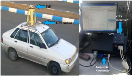
In order to evaluate the performance of the designed system, a road test was set. An instrumented car was utilized to perform the experiments as shown in Fig. 5.
The instruments used in the test include a fiber
optic gyro IMU and a GPS receiver installed on the car according to Fig. 5. The IMU consists of three orthogonal MEMS accelerometer (bias of several
milli-g) and three orthogonal fiber optic gyroscope
(gyro drift of 1.0 deg/h). To test the effect of de-noising inertial sensor data on the system results, the positioning performance of INS/GPS integration
during GPS outages is analyzed offline.
The de-noising procedure was applied to real data set collected using tactical-grade IMU. The trajectory of the test is a closed path of the Campus of Isfahan University of Technology shown in Fig. 6. It also shows the true trajectory measured by GPS for twenty minutes travelling time.
In this work, soft thresholding and threshold value obtained by Steins unbiased risk estimation method proposed by Donoho et al. [36] are used. The de-noising result shows that Daubechies 5 wavelet
filter is the best filter type used to remove the high
frequency noise. The appropriate LOD must be
Fig. 6. Road test trajectory in the Campus of Isfahan University of Technology (Google map)
selected before performing wavelet decomposition. Therefore, to select the appropriate LOD, a spectral analysis of the raw IMU data is performed. Fig. 7 shows the spectrum of kinematic and static raw data of x-axis accelerometer. The spectral analysis clearly shows that the motion dynamics is locatedat low frequenciesless than about 5 Hz. The maximum acceptable value of LOD that can be considered is level four.
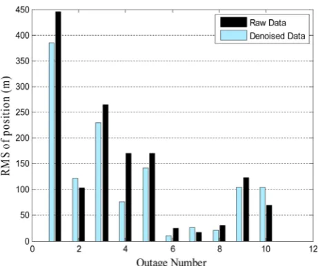
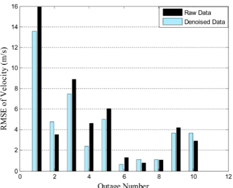
In this test, a number of 10 GPS outages were selected and the selected outage intervals are 60 seconds. Fig. 8 shows the estimated position in the horizontal (e.g. east and north) direction of the trajectory using raw and de-noised IMU signals. Root mean square of the position and velocity errors during the selected GPS outages of both raw INS/ GPS navigation and de-noised INS/GPS navigation are computed and are shown in Figs. 9 and 10,
Fig. 7. The spectrum of kinematic and static raw data of
x-axis accelerometer
respectively.
The position errors of INS/GPS integration during GPS outages are decreased mostly by removing the high frequency portion of the inertial sensor noises. The results show that total improvement of about 14% in root mean square of the position errors and about 12% in root mean square of the velocity errors are obtained using WMRA procedure. The average of the position errors at the end of the GPS outages obtained in a navigation system using de-noised IMU data was reduced by 18%. The results obtained from the practical test for travelled trajectories are summarized in Table 1.
It is not easy to compare the results of present work with those of others. Actually, comparisons between results require the same test conditions, such as, sensors used, traveled trajectory and a vehicle that performs the test. However, the test
Fig. 9. RMS of position error during GPS outages Fig. 8. Estimated positions using the raw data and
Fig. 10. RMS of velocity error during GPS outages
conditions and the results of Nassar et al. [39] are presented here. They performed two tests to evaluate the effect of de-noising inertial sensor data on the positioning performance of INS/DGPS integrated
navigation system. The first test was carried out using
a navigation-grade IMU in Laval, Quebec while the second test was performed using a tactical-grade IMU in Calgary, Alberta during DGPS outages. They chose a number of 10 DGPS outages, and the selected outage intervals were ranged from 70 sec. to
100 sec. and from 70 sec. to 180 sec. for the first and
Table. 1. Performance comparison between raw data and denoised data in integrated navigation
RMSE of Position (m)
RMSE of Velocity (m/s)
Type of Data Raw Denoised Raw Denoised
Outage No. 1 445 384 15.92 13.53
Outage No. 2 103 122 3.55 4.72
Outage No. 3 264 230 8.91 7.46
Outage No. 4 170 76 4.64 2.41
Outage No. 5 169 142 6.06 5.01
Outage No. 6 24.5 9.7 1.32 0.63
Outage No. 7 16.5 25.65 0.76 1.11
Outage No. 8 30 20.44 1.07 1.12
Outage No. 9 123 104.62 4.21 3.69
Outage No. 10 69 104.18 2.92 3.66
Mean 141.78 121.96 4.93 4.33
second test, respectively. The third and fourth levels were used for the LOD of the navigation-grade and the tactical-grade IMU data, respectively. The results show that the position errors at the end of the DGPS outages were reduced by 13%–34%.
5- Conclusion
The high-frequency noise portion of inertial data causes deterioration of position accuracy of the INS/ GPS integrated navigation system, especially during GPS outages. To overcome such a problem, a de-noising procedure based on WMRA technique has been used. Determining the exact value of LOD is very critical in the process of de-noising. In order to obtain an accurate LOD, spectral analysis of static and dynamic data was performed.
An experimental analysis was done using a tactical grade IMU installed on the car for a ring trajectory. The results of the road test show a 14% improvement in root mean square of the position errors during the selected GPS outages using WMRA de-noising technique. The average of the position errors at the end of the GPS outages obtained in a navigation system using de-noised IMU data was reduced by 18%.
6- Appendix
7- References
[1] Grewal, M. S.; Weill, L. R. and Andrews, A. P.; “Global Positioning Systems, Inertial Navigation, and Integration,” John Wiley and Sons, 2001
[2] Kalman, R. E.; “A New Approach to Linear Filtering and Prediction Problems,” ASME Trans. Ser. D: J. Basic Eng., Vol. 82, No. 1, pp. 34–45, 1960. [3] Farrell, J. A. and Barth, M.; “The Global Positioning System and Inertial Navigation,”
McGraw-Hill Professional, New York, 1999.
[4] Maybeck, P. S.; “Stochastic Models, Estimation
and control,” Academic Press, New York, Vol. 1,
1979.
[5] Skog, I. and Handel, P.; “Time Synchronization Errors in Loosely Coupled GPS-Aided Inertial
Navigation Systems,” IEEE Transactions on
Intelligent Transportation Systems, Vol. 12, No. 4, pp. 1014–1023, 2011.
[6] Shabani, M.; Gholami, A. and Davari, N.; “Asynchronous Direct Kalman Filtering Approach
for Underwater Integrated Navigation System,”
Nonlinear Dyn, Vol. 80, Nos. 1–2, pp. 71–85, 2015. [7] Wendel, J.; Schlaile, C. and Trommer, G. F.; “Direct Kalman Filtering of GPS/INS for Aerospace Applications,” International Symposium on Kinematic System in Geodesy, Geomatics and Navigation, Alberta, Canada, 2001.
[8] Qi, H. and Moore, J. B.; “Direct Kalman Filtering
Approach for GPS/INS Integration,” IEEE Trans.
Aerosp. Electron. Syst., Vol. 38, No. 2, pp. 687–693, 2002.
[9] Shabani, M.; Gholami, A.; Davari, N. and Emami, M.; “Implementation and Performance Comparison of Indirect Kalman Filtering Approaches for AUV Integrated Navigation System Using Low Cost IMU,”
ICEE, Mashhad, Iran, pp. 1–6, 2013.
[10] Chiang, K.; Aboelmagd, N. and El-Sheimy, N.; “Constructive Neural-Networks-Based MEMS/
GPS Integration Schme,” IEEE Trans. Aerospace
Electronic Syst., Vol. 44, No. 2, pp. 582–594, 2008. [11] Schwarz, K. P. and Wei, M.; “Modeling INS/GPS for Attitude and Gravity Applications,” Proceedings of the 3rd International Workshop of High Precision Navigation, Stuttgart, Germany, Vol. 95, pp. 200– 218, 1995.
[12] Ŝkaloud, J.; “Optimizing Georeferencing of
Airborne Survey Systems by INS/GPS,” Ph.D. Thesis, Department of Geomatics Engineering, University of Calgary, Calgary, Alberta, Canada, UCGE Report No. 20126, 1999.
[13] El-Rabbany, A. and El-Diasty, M.; “An Efficient
Neural-Network Model for De-noising of MEMS-based Inertial Data,” The Journal of Navigation, Vol. 57, pp. 407–415, 2004.
[14] Sifuzzaman, M.; Islam, M. R. and Ali, M. Z.; “Application of Wavelet Transform and its Advantages Compared to Fourier Transform,” Journal of Physical Sciences, Vol. 13, pp. 121–134, 2009.
[15] Grejner-Brzezinska, D.; Torh, C. and Yi, Y.; “On Improving Navigation Accuracy of GPS/INS
Systems,” Photogrammetric Engineering and Remote
Sensing, Vol. 71, No. 4, pp. 377–389, 2005.
[16] Daubechies, I.; “Orthonormal Basis of Compactly
Supported Wavelets,” Comm. Pure Applied Math.,
Vol. 41, No. 7, pp. 909–996, 1988.
System (INS) Error Model for INS and INS/
DGPS Applications,” Ph.D. Thesis, Department
of Geomatics Engineering, University of Calgary, Canada, UCGE Report No. 20183, 2003.
[18] Abdel-Hamid, W.; Osman, A.; Noureldin, A. and El-Sheimy, N.; “Improving the Performance of MEMS-based Inertial Sensors by Removing Short-Term Errors Utilizing Wavelet Multi-Resolution
Analysis,” in Proceedings of ION NTM, San Diego
CA, U.S. Institute of Navigation, pp. 260–266, 2004. [19] Bruton, A.; Schwarz, K. P. and Ŝkaloud, J.; “The
Use of Wavelets for the Analysis and De-noising of
Kinematic Geodetic Measurements,” Proceedings of
the IAG Symposia No. 121, Geodesy Beyond, The Challenges of the First Decade, Birmingham, UK, pp. 227–232, 2000.
[20] Zhang, T. and Xu, X. S.; “A New Method of Seamless Land Navigation for GPS/ INS Integrated System,” Measurement, Vol. 45, No. 4, pp. 691–701, 2012.
[21] Noureldin, A.; Osman, A. and EI-Sheimy, N.; “A Neuro-Wavelet Method for Multi-Sensor System
Integration for Vehicular Navigation,” Meas. Sci.
Technol., Vol. 15, No. 2, pp. 404–412, 2004.
[22] Burrus, C. S.; Gopinath, R. and Guo, H.; “Introduction to Wavelet and Wavelet Transforms a Primer,” Prentice Hall, 1998.
[23] Goswami, A. and Chan, K.; “Fundamentals of Wavelets: Theory, Algorithms and Applications,”
Wiley, p. 359, 1999.
[24] Ogden, R. T.; “Essential Wavelets for Statistical Applications and Data Analysis,” Birkhäuser Boston, 1997.
[25] Strang, G. and Nguyen, T.; “Wavelets and Filter Banks,” Wellesley-Cambridge Press, 1997.
[26] Buccigrossi, R. W. and Simoncelli, E. P.; “Image Compression via Joint Statistical Characterization in the Wavelet Domain,” IEEE Image Process., Vol. 8, No 12, pp. 1688–1701, 1999.
[27] Romberg, J. K.; Choi, H. and Baraniuk, R. G.; “Bayesian Tree-Structured Image Modeling Using
Wavelet-Domain Hidden Markov Models,” IEEE
Image Process., Vol. 10, No. 7, pp. 1056–1068, 2001. [28] Mallat, S. G.; “A Theory for Multiresolution Signal Decomposition: The Wavelet Representation,”
IEEE Trans Pattern Analysis and Machine
Intelligence, Vol. 11, No. 7, pp. 674–693, 1989. [29] Alnuaimy, A. N. H.; Ismail, M.; Ali, M. A. M. and Jumari, K.; “TCM and Wavelet De-noising Over an Improved Algorithm for Channel Estimations of OFDM System Based Pilot Signal,” J. Applied Sci., Vol. 9, pp. 3371–3377, 2009.
[30] Putra, T. E.; Abdullah, S.; Nuawi, M. Z. and
Nopiah, Z. M.; “Wavelet Coefficient Extraction
Algorithm for Extracting Fatigue Features in Variable Amplitude Fatigue Loading,” J. Applied Sci., Vol. 10, No. 4, pp. 277–283, 2010.
[31] Misiti, M.; Misiti, Y.; Oppenheim, G. and Poggi, J. M.; “Wavelet Toolbox for the Use with Matlab,”
The Mathworks Inc., MA, USA, 2000.
[32] Ma, X.; Zhou, C. and Kemp, I. J.; “Automated Wavelet Selection and Thresholding for PD Detection,” IEEE Electrical Insulation Magazine, Vol. 18, pp. 37–45, 2002.
[33] Li, W. and Zhao, J.; “Wavelet Based De-noising Method to Online Measurement of Partial Discharge,” Proceedings of Asia-Pacific Power and
Energy Engineering Conference, Wuhan, China, pp. 1–3, 2009.
[34] Veterli, M.; Chang, S. G. and Yu, B.; “Spatially Adaptive Wavelet Thresholding with Context Modeling for Image De-noising,” IEEE Trans. Image Process., Vol. 9, No. 9, pp. 1522–1531, 2000.
[35] Misite, M.; Misite, Y.; Oppenheim, G. and Poggi, J. M.; “Wavelet Toolbox: Computation, Visualization
and Programming: Version 2,” Mathworks Inc.,
California, 2002.
[36] Donoho, D.; Iain, L. and Johnstone, M.; “Adapting to Unknown Smoothness via Wavelet
Shrinkage,” Journal of the American Statistical
Association, Vol. 90, No. 432, pp. 1200–1244, 1995. [37] Titterton, D. H. and Weston, J. L.; “Strapdown Inertial Navigation Technology,” Peter Peregrinus, UK, 1997.
[38] Brown, R. G. and Hwang, P. Y. C.; “Introduction to Random Signals and Applied Kalman Filtering:
With MATLAB Exercises and Solutions,” Wiley,
New York, Vol. 1, 1997.
![Fig. 1. Signal Decomposition by the Discrete Wavelet Transform [12]](https://thumb-us.123doks.com/thumbv2/123dok_us/17139.2001731/3.595.320.559.81.248/fig-signal-decomposition-discrete-wavelet-transform.webp)
![Fig. 2. Wavelet multi-resolution analysis (considering three levels of decomposition) [12]](https://thumb-us.123doks.com/thumbv2/123dok_us/17139.2001731/4.595.45.273.588.754/fig-wavelet-multi-resolution-analysis-considering-levels-decomposition.webp)