Iranian Journal of Electrical and Electronic Engineering, Vol. 16, No. 1, March 2020 13
A Hybrid Switching Technique for Single-Phase AC-Module
PV System to Reduce Power Losses and Minimize THD
H. Toodeji*(C.A.)
Abstract: This paper proposes a hybrid switching technique for a domestic PV system with AC-module architecture. In this PV system, independent control of PV modules, which are directly connected to DC terminals of a single-phase cascaded multilevel inverter, makes module-level MPPT possible to extract maximum available solar energy, especially in partial shading conditions. As one of the main contributions, the proposed hybrid method employs a fundamental-based switching technique to decrease power losses, which directly affect the efficiency of solar energy conversion. In addition, fast dynamic response of the introduced hybrid technique lets the PV system to harvest more power in partial shading conditions. Producing a waveform with minimized THD in steady-state conditions is another advantage of the proposed switching technique. In this paper, the advantages of the proposed hybrid method are verified by the simulation of a test PV system with both conventional SPWM and proposed switching techniques in MATLAB/Simulink under various partial shading conditions.
Keywords: Cascaded Multilevel Inverter, Fundamental Frequency Switching Technique,
Single-Phase PV System, Switching Losses, THD Minimization.
1 Introduction1
OWADAYS, small-scale PV systems are
increasingly installed all around the world from isolated rural spaces to residential areas [1, 2]. To harvest the highest possible solar energy from these PV
systems, different maximum power point
tracking (MPPT) methods are introduced. Conventional MPPT methods can correctly find the optimal operating point when all PV modules experience the same conditions [3]. However, they unable to track the globally optimal point in mismatched operating conditions in which multiple local optima will be arisen [4]. As a result of the suboptimal operation of some PV modules, the total harvested power is significantly affected [5]. In addition, the creation of hot spots in the suboptimal PV modules results in their fast deterioration
Iranian Journal of Electrical and Electronic Engineering, 2020. Paper first received 27 September 2019, revised 14 November 2019, and accepted 16 November 2019.
* The author is with the Electrical Engineering Department, Yazd University, Yazd, Iran.
E-mail: toodeji@yazd.ac.ir. Corresponding Author: H. Toodeji.
[6].
The mismatch in operating conditions is mainly caused by nonuniform illumination in which some PV modules experience different solar radiation, partially or
totally [7]. For instance, building-integrated
photovoltaic (BIPV) systems endure such conditions, because PV modules may be installed on a curved surface [8]. Besides, surrounding obstacles in urban environments or shading of one PV module to another in compact installations often lead to partial shading conditions. In addition, there are environmental phenomena such as bird droppings and moving clouds, as fixed and moving shadings, respectively, that block/decrease received sunlight by some PV cells for a while [9].
To extract maximum power and prevent damage to PV modules in partial shading conditions, various methods have been proposed. These methods can be categorized in the following four groups: utilizing developed MPPT techniques [10], changing the configuration of PV arrays [11], using appropriate architectures [12-14], and employing novel converter topologies [15]. In AC-module architecture, each PV module is connected to its own microinverter, so module-level MPPT can be carried out to harvest more
N
Iranian Journal of Electrical and Electronic Engineering, Vol. 16, No. 1, March 2020 14
power in partial shading conditions. It is worth mentioning that this microinverter can be the stages of a cascaded multilevel inverter.
In some PV systems with AC-module architecture, a DC-DC converter, also known as power optimizer, is employed beside or merged in each microinverter to perform module-level MPPT [16, 17]. It is worth mentioning that more than 55% of domestic PV systems in the USA have utilized various combinations of local power optimizer and microinverter, known as module-level power electronics (MLPE), as one of the fastest growing markets in the solar industry, in 2014 [18]. However, some studies have introduced various module-level MPPT structure with no need for local power optimizers [12]. Elimination of local power optimizers reduces the size, cost and control complexity of PV systems and also increases the reliability as well as the efficiency of the PV system.
In the present paper, a hybrid switching technique is proposed for a single-phase PV system with the cascaded multilevel inverter. In this AC-module architecture, PV modules are directly connected to the DC terminals of multilevel inverter without any DC optimizer. One of the main contributions of the hybrid switching technique is power losses reduction that improves the efficiency of the solar energy conversion system. This purpose is obtained by employing a fundamental frequency-based switching technique, however slower dynamic response of such techniques may inversely affect total harvested power in comparison with conventional SPWM. To deal with this concern, both SPWM and fundamental frequency techniques are combined in the hybrid technique to improve the dynamic response. As another contribution, the THD value of the produced waveform in steady-state conditions is minimized to meet the limits of available harmonic standards.
This paper is organized as follows; the configuration of the single-phase AC-module PV system is presented in Section 2 and then, the proposed hybrid switching technique for this PV system is overviewed in the next section. Section 4 is dedicated to explaining the modified decoupled current controller and a detailed description of the proposed two-step hybrid switching technique can be found in Section 5. Section 6 is devoted to the simulation of a test PV system with both conventional SPWM and proposed hybrid switching techniques in MATLAB/Simulink under various partial shading conditions. Comparing the obtained results can verify the advantages of the hybrid switching technique over conventional SPWM.
2 Configuration of Single-Phase AC-Module PV System
The configuration of a single-phase PV system with the AC-module structure is presented in Fig. 1. It is seen that each PV module is directly connected to a specific
H-bridge #1
H-bridge # n IPV,1
IPV,n
RS LS
AC Grid
einv i vGrid
+ VDC,1
--+ VDC,n
--Fig. 1 Single-phase AC-module PV system.
H-bridge of the cascaded multilevel inverter. Moreover, the multilevel inverter is connected to the single-phase AC grid through a first-order filter decreasing the harmonic content of injected current. In spite of the fact
that RS and LS represent the resistance and inductance of
harmonic filter, respectively, Thevenin's impedance of the AC grid at point of common coupling (PCC) are also considered in this impedance. It is noteworthy that other higher-order harmonic filters, like LC and LCL, can also be utilized instead of the present first-order filter, considering the limits of a specific harmonic standard.
3 An Overview of the Proposed Hybrid Switching Technique
In this section, the proposed two-step hybrid switching technique for the presented AC-module PV system is overviewed. As expected, the switching technique should consider both steady-state and transient conditions. The main concern of steady-state condition is power losses reduction as well as THD minimization, so a fundamental frequency-based switching technique is employed instead of the conventional SPWM. In addition, the proposed switching technique should also be able to utilize a simple MPPT method, such as standard perturb & observe (P&O), to perform module-level MPPT in the PV system with AC-module structure.
In the standard P&O method, which is described by the discrete-time dynamic model in (1) and presented in
Fig. 2, the variation of PV voltage (ΔVPV) and power
(ΔPPV) are employed to produce controlled perturbation
command.
1 PV PV 1 .sgn
PV PV 1
x k x k V k V k P k P k (1)
where sgn represents the signum function and x(k) an
internal perturbation variable to generate the MPPT control signal [19].
Obviously, a fundamental frequency-based technique needs more time to perform this MPPT method, since it cannot quickly change PV voltages. Therefore, employing this switching technique for both steady-state and transient conditions can inversely affect the
Iranian Journal of Electrical and Electronic Engineering, Vol. 16, No. 1, March 2020 15
dynamic response. Moreover, ambient conditions may also be varied during such a time-consuming procedure for some PV modules due to a transient shadow such as fast-moving clouds on a windy day.
To improve the dynamic response, the conventional SPWM technique is employed in step 1 having fast MPPT. However, additional power losses due to utilizing the SPWM technique can be neglected, since partial shading conditions do not happen frequently and also new MPPs can be quickly found. Moreover, fast MPPT decreases the suboptimal operation interval of partially shaded PV modules, so the harvested power as well as the efficiency of the PV system increase. Due to the inherent oscillatory response of the
standard P&O method [19], power variation (ΔP)
smaller than εp is considered as finishing of MPPT
procedure in step 1, as seen in Fig. 3. Upon finding the optimal operating point, step 2 starts and the switching technique is returned to the fundamental frequency-based technique to reduce the power losses. It should be noted that the required switching angles to regulate modules’ voltages at their recently found optimal values are quickly calculated in substep 1 before changing the switching technique. These switching angles may result in waveforms with high THD amounts since there is no control on THD value. Finding optimal switching angles for THD minimization as well as DC voltage regulation in substep 2 is a time-consuming procedure. On the other hand, continue to operation in SPWM until the end of this optimization procedure increases the power losses. Thus, the proposed switching technique employs SPWM only for finding MPP and then immediately returns to the fundamental frequency-based technique with suboptimal switching angles until the calculation of optimal angles I substep 2.
In addition to finalizing step 1, more attention to Fig.
3 clears that modulation index changes (ΔM) bigger
than εM can also activate step 2. Such change may
happen solely due to variations of reactive power
Start
ΔPpv > 0 Measure Vpv & Ipv
Calculate Ppv
ΔPpv = 0 Yes Yes No No
ΔVpv > 0 ΔVpv > 0
x = x + Δx
Update Vpv & Ipv
Return
x = x - Δx x = x + Δx
x = x - Δx
Yes
Yes No No
Fig. 2 Flowchart of the standard P&O method [19].
reference in the modified decoupled current controller.
Therefore, those conditions with ΔM bigger than εM and
ΔP smaller than εp are directly conducted to step 2
preventing unnecessary activation of step 1.
4 Modified Decoupled Current Control
The lowest level of the hierarchical controller for the PV system, which generates gate signals for multilevel inverter, is commanded by a modified decoupled current controller as its upper control level. In the well-known structure of the decoupled current controller, which is
Start
ΔP > ɛp
Measure P & M
Find optimal DC voltages
PWM switching technique
Current controller
Calculating switching angles
Fundamental Frequency switching
technique
Is Minimization finished? Find optimum
waveform
Fundamental Frequency switching
technique With new angles
Step 2 Step 1
ΔM > ɛm
or
ΔP > ɛp
THD minimization
Yes
Yes
Yes
Yes No
No
No
No
Substep 1
Substep 2
ΔP < ɛp
Fig. 3 Flowchart of the proposed two-step hybrid switching technique.
Iranian Journal of Electrical and Electronic Engineering, Vol. 16, No. 1, March 2020 16
commonly used in three-phase systems, derived
equations are transformed from stationary abc to
quadratic rotary dq frame. This transformation can be
applied to those systems with at least two independent
phases, so dq model of the present single-phase circuit
cannot be directly obtained. To solve this problem, an imaginary orthogonal circuit, which is constructed at the basis of the real circuit, can be assumed as the second independent circuit. The components of this imaginary
circuit are similar to that of the real circuit, but with 90o
phase-shifted state variables. One may consider a specific delay in the real circuit to achieve the desired phase-shift, but this delay inversely affects dynamic response [20]. Differentiation, as an alternative solution, can also result in the desired phase-shift with no impact
on dynamic performance [21]. For instance, xI(t) in (2)
is a state variable of an imaginary circuit, which is
obtained by differentiation of xR(t), as a state variable of
real single-phase circuit:
sin cos R R R I I I Rx t A t
d x t
x t A t
dt A A (2)
where AR and AI are the amplitude of real and imaginary
state variables, respectively, ω is the fundamental
angular frequency in rad/sec and φ is the initial phase
angle in rad. Also, the amplitude of the imaginary state
variable is multiplied by 1/ωafter differentiation.
Now, the given transformation matrix T in (3) can be
utilized to determine d- and q-axis components of
single-phase state variables in dq coordinates, which are
respectively shown by xd and xq in (3).
sin cos . , sin cos cos sin sin cos R d R I q A t xT A A
x t t t T t t (3)
Applying KVL to the AC side of the PV system in Fig. 1 results in the following equation:
0
inv S S Grid
di
e L R i v
dt
(4)
here, vGrid is the AC grid voltage at PCC and einv
represents the produced voltage of the multilevel
inverter. Transforming this equation to dq coordinates
by (3) leads to the following equations:
, Grid, , Grid,q
1 1
1 1
S
d d q inv d d
S S S
S
q q d inv q
S S S
R d
I I I E V
dt L L L
R d
I I I E V
dt L L L
(5)
where, Einv,d and Einv,q are d- and q-axis components of
multilevel inverter’s voltage, respectively, VGrid,d and
VGrid,q represent d- and q-axis components of AC grid
voltage, and correspondingly, Id and Iq are d- and q-axis
current components. In the dq rotary frame, active and
reactive power in the AC side of the PV system can be defined by the following equations:
Grid, Grid, Grid, Grid,q | | 0 Grid, Grid,q 2 1 2 1 2 2 d q dd d q
V V
V
d q d q
P I
P V I V I V
Q
Q V I V I I
V (6)
Aligning d-axis of dq rotary frame to VGrid,d results in
VGrid,q = 0 and VGrid,d = |V| in which |V| is the amplitude
of AC grid voltage. As a result, (6) shows that the active and reactive powers can be independently controlled by
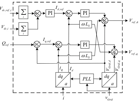
d- and q-axis currents, respectively. Fig. 4 presents the
block diagram of the modified decoupled current
controller at the basis of derived equations in dq
coordinates. It can be seen that the reference of active power, specified by a PI controller, is dedicated to the regulation of the summation of DC voltages. Also, the
reactive power reference (Qref) is commanded by a
higher control level having an appropriate power factor correction.
5 Proposed Two-Step Switching Technique
After calculation of reference voltages in dq
coordinates (Vref,d and Vref,q) by the modified decoupled
current controller, these values are given to the two-step hybrid switching technique, as Fig. 5 shows. In this section, two parallel steps of the proposed technique, which are overviewed in section 3, are described in detail.
5.1 Step 1: Fast MPPT by SPWM Switching Technique
In steady-state conditions, the PV system is governed by a fundamental frequency-based switching technique.
+- PI i
i
+- PI S L PI S L q I refQ ×÷ +
-, q ref I , d ref I + + -+ -, ,
dc ref i
V , dc i V Grid v i a dq PLL a dq d I , G rid d V , G rid q V , ref q V ,d ref V
Fig. 4 The block diagram of the modified decoupled current controller.
Iranian Journal of Electrical and Electronic Engineering, Vol. 16, No. 1, March 2020 17 ,1, dc ref V P&O MPPT method ,1 PV I ,1 dc V D e c o u p le d c u rr e n t c o n tr o lle r , ,
dc n ref
V P&O MPPT method ,n PV I ,n dc V ,1 dc V , dc n V ref Q , ref q V ,d ref V dq , M M
,2, dc ref V +- PI ,2 dc V ,n, dc ref V +- PI ,n dc V i
+- M1
2 M n M Grid v i P h a s e s h if te d S P W M Gate signals
Fig. 5 Block diagram of step 1.
, ,
dc i ref
V D e c o u p le d c u rr e n t c o n tr o lle r , dc i V ref Q , ref q V ,d ref V dq ,
M M
i Grid v i M u lt ile v e l in v e rt e r C a lc u la ti o n o f s w it c h in g a n g le s , dc i V F in d o p ti m u m w a v e fo rm Decision Enable out P T H D o p ti m iz a ti o m G e n e ra ti n g p a tt e rn n n n n n m Substep 1 Substep 2
Fig. 6 Block diagram of two parallel substeps of step 2.
Upon a change in ambient conditions such as total or partial shading, step 1 with the presented block diagram in Fig. 5 activates to find new MPP of each PV module. Since the utilized SPWM switching technique increases the power losses, inappropriate activation of this step should be avoided. Therefore, those active power
changes higher than εp, as the sign of happening a
variation in ambient conditions, only can activate step 1 (see Fig. 3).
The presented block diagram of step 1 in Fig. 5, inspired by [21], shows that the MPP of each PV module is separately found by the standard P&O method. Also, it is seen that MPPT control signals as well as commanded reactive power are given to the
modified decoupled current controller for generating d-
and q-axis voltage references. Considering (7) clears
that these two reference values are utilized to synthesize
the modulation index (M) and the voltage phase angle
(δ) for active and reactive power control.
2
2, , 1 ,
, ,
1
,
ref d ref q ref q
n
ref d dc i
i
V V V
M tg V V
(7)Afterward, the obtained modulation index (M) is
employed besides the PI controller of i-th DC voltage to
produce modulation index of i-th stage of cascaded
multilevel inverter (Mi) for i = 2, …, n. However, the
first modulation index (M1) is obtained by (8), since the
summation of Mi for i = 1, …, n should be equal to the
calculated M in (7).
1
2
n
i i
M M M
(8)5.2 Step 2: Power Losses Reduction and THD Minimization
At the end of step 1, all PV modules, regardless of experiencing partial shading conditions, operate in their MPPs, so the fundamental frequency-based technique can be utilized again to reduce power losses and minimize THD. As it is specified in Figs 3 and 6, two parallel substeps begin with activation of step 2, so the detailed explanation of these substeps is presented in the following.
5.2.1 Substep 1: DC Voltage Regulation
As it was mentioned, the modified decoupled current controller could not independently regulate each PV
Iranian Journal of Electrical and Electronic Engineering, Vol. 16, No. 1, March 2020 18
module at its optimal voltage. Therefore, a
supplementary control system, inspired by [22, 23], is proposed to independent regulation of DC voltages. At first, the Fourier analysis of produced voltage by a
cascaded multilevel inverter with n unequal DC sources
is considered:
1
,1 1 ,
sin ,
4
.cos .cos ,
0 ,
o k
k
dc dc n n
k
V t V k t
V k V k odd k
V k even k
(9)where, Vk represents the amplitude of k-th voltage
harmonic, Vdc,i and θi for i = 1,…, n are the voltage of i
-th unequal DC source and switching angle, respectively. By considering the fundamental component of this
waveform, modulation index (M) can be defined by
(10), as the normalized value of the fundamental component:
,1 1 ,
1
, ,
1 1
4
.cos .cos
dc dc n n
n n
dc i dc i
i i V V V M V V
(10)As it has been introduced in [22], the voltage of each DC capacitor in the cascaded multilevel inverter can be regulated by its charging control. In the PV system, the generated power of each PV module is injected to its relevant DC capacitor and then delivered to the AC system, after subtraction of conduction as well as switching losses. Therefore, the voltage of each DC capacitor can be easily regulated by controlling its delivered power. Since a fundamental frequency-based switching technique is employed and DC voltages should be fixed at their optimal values, charge control can be obtained through switching angles.
With the assumption of a harmonic-free current in AC side of the multilevel inverter due to an appropriate
harmonic filter, applying KCL at DC side of i-th
H-bridge results in (11):
, , , , , , , sin ,c i PV i loss i inv PV i inv
loss i
inv m loss i
dc i
I I I I I I
P
I I t I
V
(11)
where, Ipv,iis generated current of i-th PV module, Ic,i
and Ploss,i are representative of capacitor current and
power losses of i-th H-bridge, respectively. Moreover,
the phase angle between the grid voltage and current is
shown by φ and Im is the amplitude of the AC side
current of multilevel inverter (Iinv). To obtain equivalent
losses current (Iloss,i), the calculated power losses of each
H-bridge is divided by its relevant DC voltage. Since the power loss of each H-bridge is supplied by its connected PV module, the net injected current is
specified by I'pv,i. It is worth mentioning that the
introduced method in [24] is employed in the present study to calculate conduction and switching power losses. In this method, power losses are calculated at the basis of datasheet values and/or experimental measurements with minimum effort, high accuracy and little impact on the simulation time.
The average charge of i-th DC capacitor can be
obtained by:
' , 0 1 sin Ti PV i m
Q I I t dt
T
(12)Due to the operation of i-th H-bridge, Iinv flows into its
DC and AC sides for [θi, π-θi] and [π+θi, 2π-θi],
respectively. For other intervals of the switching cycle, short-circuiting of AC side results in isolation of DC capacitor from this side. Therefore, (12) can be extended to (13):
, 2 0 , sin 1 1 2 sin 2 cos cos i i i i m Ti PV i
m
PV i m i
I t d t
Q I dt
T
I t d t
I I
(13)Considering the effect of power losses as an independent branch in (11) leads to lossless H-bridges. Thus, power balance equation can be written for the single-phase cascaded multilevel inverter. In this balance equation, delivered active power to the AC grid
(Pout) should be equal to the total extracted power of PV
modules minus total power losses.
1 , j , , j , j
1 , , j 1
, , j 1 , j 1 1 cos 2 cos 4 cos n
out m PV dc j loss dc
j
n
PV j dc j
n
PV j dc j
m n
dc j
j
P V I I V I V
I V I V I V
(14)Substitution of (14) in (13) results in (15):
, , j 1 , , j 1 cos 2 cos n
PV j dc j
i PV i n i
dc j j I V Q I V
(15)In steady state conditions, average charge of DC capacitors should be equal to zero having constant DC voltages:
Iranian Journal of Electrical and Electronic Engineering, Vol. 16, No. 1, March 2020 19
, ,
, j1
2 cos cos 0, 1, ,
n
PV i j PV j i dc
j
I I V i n
(16)
Beside these charging equations, desired modulation index, defined by (10), should also be satisfied. Therefore, first equation of (16) is substituted by (10) to
form a system of n-equation with n switching angles as
their unknown variables. Solving this system of
equations guarantees regulation of M as well as Vdc,i for
i = 2,…, n at their desired values, and Vdc,1 can be easily
controlled by regulation of DC voltages’ summation through the modified decoupled current controller. It is worth mentioning that this system of equations can be
simply turned to linear equations by considering cos(θi)
instead of θi for i = 1,…, n as their variables.
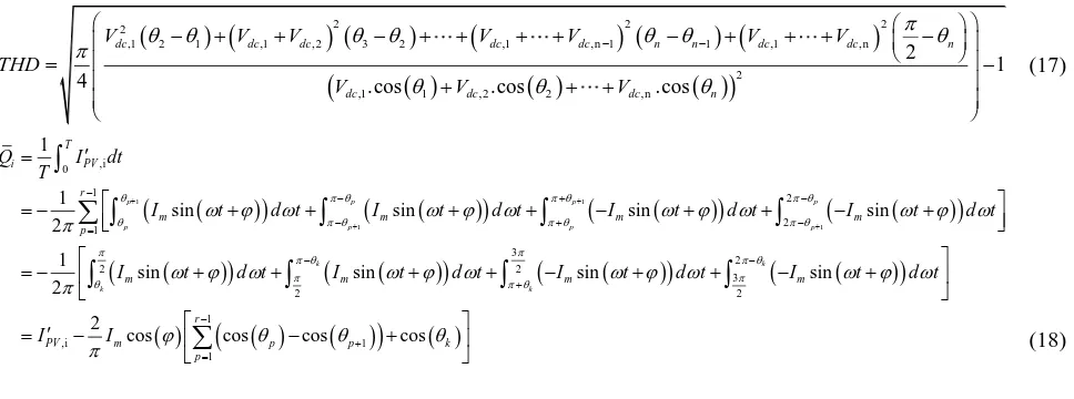
Now, one may try to minimize the THD of obtained waveform with these switching angles. However, the given THD formula in (17) shows that no unspecified switching angles remains for employing in THD minimization procedure [25]. Indeed, THD value is completely specified by the present optimal DC voltages as well as reactive power reference.
5.2.1 Substep 2: THD minimization
The given THD formula in (17) has no degree of freedom for THD minimization, so substep 2 with the presented flowchart in Fig. 7 is proposed to minimize
THD value. In this flowchart, optimal DC voltages (Vdc,i
for i = 1,…, n) are sorted from smallest to largest and
then, their combinations C(n, i) for i = 1,…, n are
obtained. Among achieved sets of DC voltages, the elements of those combinations with cardinality of at least 2 are separately summed. By sorting summation results as well as those combinations with cardinality of
1 from smallest to largest, a set of V'i for i = 1,…, k is
obtained. This can produce a k-level waveform with k
switching angles, as shown in Fig. 8. Since DC voltages
as well as reactive power can be regulated by n
switching angles, k-n switching angles remain that can
be utilized as degrees of freedom for THD minimization.
It is worth mentioning that the equality of some DC
voltages decreases the number of obtainable voltage levels. Accordingly, Equality of all DC voltages, as the worst case, results in a waveform without the capability of THD minimization.
Now, similar to substep 1, the average charge of each DC capacitor should be set to zero. Considering Table 1, which specifies the number of repetitions for each DC voltage in different combination sets, may help to write charging equations. It is assumed that the assigned
numbers to DC voltages indicate their rank, so Vdc,1 and
Vdc,n have the smallest and largest values, respectively.
Regarding the number of repetitions for i-th DC
voltage in different combination sets, the charging
equation of i-th DC capacitor can be obtained by (18).
, , ,
1 2
n n n
n
, , , ,n
dc i dc
V V
Receiving
Summation of each set’s
members Selecting
Sorting results from smallest to
largest
Forming THD formula &
balancing equations (20)
Fig. 7 Flowchart of substep 2.
2 2 2
2
,1 2 1 ,1 ,2 3 2 ,1 ,n 1 1 ,1 ,n
2
,1 1 ,2 2 ,n
2
1
4 .cos .cos .cos
dc dc dc dc dc n n dc dc n
dc dc dc n
V V V V V V V
THD
V V V
(17)
1 1
1 1
,i 0
1
1 2
2
2
2 2
3
1 1
sin sin sin sin
2 1
sin sin sin sin
2
p p p p
p p p p
k
k k
T
i PV
r
m m m m
p
m m m m
Q I dt
T
I d t I d t I d t I d t
I d t I d t I d t
t t t t
t t t I
1
,
1
1
2 2
i
3
2
cos cos cos cos
k
p p
r
PV m
p
k
d t
I I
t
(18)
Iranian Journal of Electrical and Electronic Engineering, Vol. 16, No. 1, March 2020 20
1
2
2
' 1
V
' 2
V inv e
t
' 1
k V
'
k V
~ ~
1
k k
Fig. 8 The produced staircase waveform in substep 2.
Table 1 Repetitions of each DC voltage in the obtained combination sets.
Number of repetitions for each DC voltage The value of voltage
levels Number of
voltage levels & switching angles
1 Vdc,1, …, Vdc,n
1 n
n-1 (Vdc,1+Vdc,2), …,
(Vdc,n-1+Vdc,n)
2 n
1 2
2 n n (Vdc,1+Vdc,2+Vdc,3), …,
(Vdc,n-2+ Vdc,n-1+Vdc,n)
3 n
1 Vdc,1+…+Vdc,n
n
n
where, θk is the last and bigger switching angle and r
indicates the repetitions of each DC voltage. Similar to (14), applying active power balance between AC and DC sides of PV system results in (19)
, , j 1
,
, j 1
1
1 1
2 cos
cos cos cos
n
PV j dc j
i PV i n
dc j
j
r
p p k
p
I V
Q I
V
(19)
Setting these charging equations to zero in steady state
conditions form a system of n-equation with k switching
angles as their unknown variables in (20):
' '
,i , j
1
, j
1 1
1
2 cos cos
0
cos cos cos
for 1, ,
PV j PV i
n r
dc
j p p k
p
I I
V
i n
(20)
Due to higher number of variables in comparison with equations, no unique solution set can be found for (20). However, these extra switching angles give the
opportunity of performing THD minimization
procedure, in contrast with substep 1. Therefore, an optimization problem with given THD formula in (21) as its objective function is formed.
The equality constraints of this problem consist of charging equations in (20) for i = 2, …, n as well as defined modulation index in (10). It is worth mentioning
that charge equation for i = 1 in (20) can also be
considered along with other equality constraints when enough switching angles are available for THD minimization.
6 Simulation Results
In this section, the validity of proposed hybrid technique is confirmed by the simulation of a test PV system with both proposed and conventional SPWM [21] switching techniques in MATLAB/Simulink under various partial shading conditions. It should be remembered that the conventional SPWM is employed in step 1 of the proposed switching technique. Moreover, considering given parameters in Table 2 shows that the test PV system with AC-module architecture needs more than three sets of H-bridge & PV module to meet grid voltage level. Since increasing the number of these sets results in many figures, it is assumed that a string of three series PV modules is connected to each H-bridge.
2 2 2 2
' ' ' '
1 2 1 2 3 2 1 1
2
' ' ' ' '
1 1 2 1 2 1
2
1
4 .cos cos .cos
k k k k k
k k k
V V V V
THD
V V V V V
(21)
Table 2 The parameters of PV test system.
Grid Voltage 220 V, 50 Hz
Each PV module at STC (Trina Solar TSM-250PA05.08) [26] Open circuit voltage 37.6 V Short circuit current 8.55 A
Nominal power 249.86 W
Cascaded multilevel inverter
Number of H-bridges (stages) 3
IGBT Module (MG1215H-XBN2MM) [27] 1200 V, 15 A
Thermal resistance Case to sink 0.02 K/W
Sink to ambient 0.072 K/W
DC capacitor Ci 3 mF
Switching frequency (SPWM technique) fsw 16 kHz
Harmonic filter 16 mΩ, 4 mH
Iranian Journal of Electrical and Electronic Engineering, Vol. 16, No. 1, March 2020 21
6.1 Simplifying Formulas
In the previous section, general formulas to calculate appropriate switching angles in the both substeps of step 2 are derived. Now, these formulas are simplified for the test PV system, which includes a three-stage single-phase multilevel inverter. In the substep 1, three optimal DC voltages, specified in step 1, produce a
7-level waveform with three switching angles.
Considering charging equations of DC capacitors No. 2 and 3 as well as the modulation index formula result in a system of three equations with three unknown switching angles in (22).
All switching angles are completely specified by solving this system of equations, so presented THD formula in (23) results in a definite value without the possibility of THD minimization. If a partial shading condition leads to three different optimal DC voltages, performing substep 2 leads to a 15-level waveform with seven switching angles. Since there are small differences between the derived formulas for two parallel substeps of the step 2, simplified formulas of substep 2 are not mentioned here.
6.1 Partial Shading Condition
At the beginning, all PV modules receive uniform
solar radiation (1000W/m2) and operate in same
ambient temperature (25oC) (see Fig. 9). Moreover, it is
assumed that three PV modules of each string, which is connected to one H-bridge of the three-stage multilevel inverter, experience same conditions. In the presented
figures of this section, each string is nominated by PVi
for i = 1, 2, 3.
Due to receiving similar solar radiation by all PV
strings before t = 0.1sec., operation of modules in same
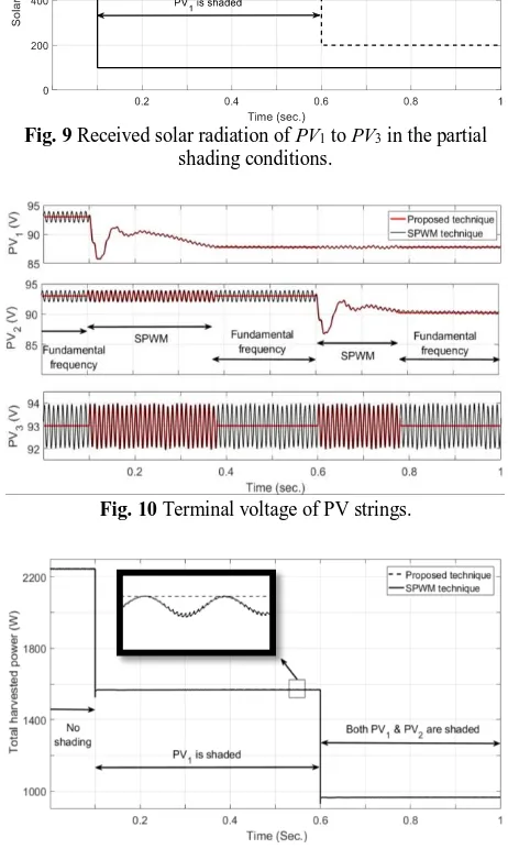
optimal DC voltages can be seen in Fig. 10. Moreover, a voltage ripple can be distinguished in the conventional technique as a result of continuous operation of the standard P&O method. These ripples can be compared with the smooth voltages of the proposed switching technique in which unnecessary operation of MPPT system is prevented. Fig. 11 shows that these voltage ripples affect the harvested power of PV modules.
Since three DC voltages are equal before t = 0.1sec.,
the three switching angles of produced 7-level
Fig. 9 Received solar radiation of PV1 to PV3 in the partial shading conditions.
Fig. 10 Terminal voltage of PV strings.
Fig. 11Total harvested power with conventional and proposed switching techniques.
,1 1 ,2 2 ,3 3 ,1 ,2 ,3
,2 ,1 1 ,1 ,1 ,2 ,2 ,3 ,3 2 ,2 ,3 3
,3 ,1 1 ,3 ,2 2 ,1 ,1 ,2
4
.cos .cos .cos
2 cos 3 cos 2 cos 0
2 cos 2 cos
dc dc dc dc dc dc
PV dc PV dc PV dc PV dc PV dc
PV dc PV dc PV dc PV
V V V M V V V
I V I V I V I V I V
I V I V I V I V
dc,2 3IPV,3 Vdc,3
cos3 0
(22)
2 2
2
,1 2 1 ,1 ,2 3 2 ,1 ,2 ,3 3
2
,1 1 ,2 2 ,3 3
2
1
4 .cos .cos .cos
dc dc dc dc dc dc
dc dc dc
V V V V V V
THD
V V V
(23)
Iranian Journal of Electrical and Electronic Engineering, Vol. 16, No. 1, March 2020 22
waveform cannot be increased by the proposed method in substep 2. However, the presented THD value in Fig. 12 is still smaller than that of the conventional SPWM. In addition, Fig. 13 clears that the proposed hybrid switching technique can expectedly reduce power losses in comparison with conventional SPWM. It is worth mentioning that the presented curves in the datasheet of the utilized IGBT module are employed for calculation of conduction as well as switching losses.
At t = 0.1sec., PV1 experiences an exaggerative
transient shadow, which decreases its received solar
radiation to 100W/m2. The consequent reduction of
harvested power activates step 1 of the proposed switching technique finding optimal DC voltages for
PV1 to PV3. Fig. 10 shows that the optimal voltage of
partially shaded PV1 is found during 0.2 seconds, while
no new optimal voltages are found for PV2 and PV3.
Since step 1 employs the SPWM technique, both conventional SPWM and proposed switching techniques result in similar voltage ripples. In addition, increasing THD value as well as power losses can be seen in Figs. 12 and 13, respectively.
It is worth mentioning that steadily decrement of power losses during this interval, which occurs for both techniques, is due to the reduction of total harvested power in the present partial shading condition. Moreover, due to temperature dependence of power losses as well as large time-constant of heat transfer systems, slow dynamic response can be seen for both
techniques in
Fig. 12 THD of produced voltage with conventional and proposed switching techniques.
Fig. 13 Total power losses of the test PV system with conventional and proposed switching techniques.
Fig. 13. In addition, different initial junction
temperatures can describe the reason for the large difference in power losses between conventional and proposed methods during step 1, when both switching techniques employ conventional SPWM. Besides, Figs 10 and 12 show that the step 1 lasts only for short-time intervals, so the junction temperature in the proposed switching technique cannot reach to those higher temperatures in the conventional SPWM.
Upon finding optimal voltages, appropriate switching angles to regulate DC voltages, as well as modulation index, are immediately calculated by substep 1. In consequence, Fig. 14 shows that the utilized switching technique is changed from SPWM to the fundamental frequency-based technique. Besides, substep 2 is also in progress to obtain a waveform with higher number of switching angles and lower THD value. Fig. 14 shows that after a few cycles, the optimization procedure finishes and as a result, an eleven-level voltage with five switching angles is obtained for the steady-state condition. Fig. 12 reveals that the THD value of the produced voltage is significantly reduced. Comparing these results with those of conventional SPWM in Figs. 12 and 13 verify the superiority of the proposed hybrid switching technique.
At t = 0.6sec., PV2 experiences a partial shading, and
its received solar radiation is decreased to 200W/m2.
The consequent change in the extracted power activates step 1 of the proposed switching technique and Fig. 10 shows that optimal DC voltages are quickly found at
t = 0.7sec., similar to the conventional SPWM. Upon
finding optimal DC voltages and activation of the
(a)
(b)
Fig. 14 Produced voltage by the proposed switching technique besides its zoomed figure.
Iranian Journal of Electrical and Electronic Engineering, Vol. 16, No. 1, March 2020 23
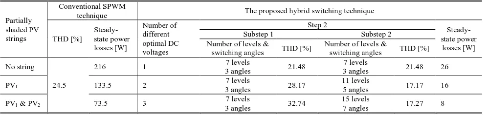
Table 3 The simulation results of both switching techniques under various partial shading conditions.
Partially shaded PV strings
Conventional SPWM
technique The proposed hybrid switching technique THD [%]
Steady-state power losses [W]
Number of different optimal DC voltages
Step 2
Steady-state power
losses [W]
Substep 1 Substep 2
Number of levels &
switching angles THD [%]
Number of levels &
switching angles THD [%] No string
24.5
216 1 7 levels
3 angles 21.48
7 levels
3 angles 21.48 26
PV1 133.5 2
7 levels
3 angles 28.17
11 levels
5 angles 17.17 16 PV1 & PV2 73.5 3 3 angles 7 levels 32.74 15 levels 7 angles 17.27 8
step 2, the utilized switching technique is returned to the
fundamental frequency-based technique and
consequently, a 7-level output waveform is produced. By finalizing optimization procedure in substep 2 and estimation of optimal switching angles, Figs. 12 and 14 reveal that a 15-level waveform with THD = 17.27% is produced. Comparing with the previous partial shading condition, three different optimal DC voltages are obtained here. Therefore, a waveform with higher number of levels and lower THD value has been achieved. Moreover, Fig. 13 presents lower power losses for both techniques, since the total harvested power is reduced in this new condition. Besides, it is seen that the response of conventional technique against this new-happened partial shading is similar to the
previous condition, which occurred at t = 0.1sec.
For the sake of comparison, the obtained results of both proposed and conventional switching techniques under mentioned partial shading conditions are summarized in Table 3. This table presents the outstanding ability of the proposed hybrid switching technique to reduce the power losses and consequently, increase the solar energy conversion efficiency. Moreover, it is seen that the THD minimization ability of the proposed switching technique is increased by the intensity of partial shading conditions. However, there is no control over the THD value when all PV modules experience the same ambient conditions and operate in similar optimal DC voltages.
It should be noted that the THD value for conventional SPWM changes in accordance with variation of optimal voltage of PV modules. However, small changes in PV modules’ optimal voltages lead to a trivial variation of THD value in Fig. 12, so a fixed THD amount is brought in Table 3 for the conventional SPWM.
7 Conclusion
In this paper, a hybrid switching technique is introduced for a single-phase domestic PV system with AC-module architecture. In this PV system, PV modules are directly connected to DC terminals of a cascaded multilevel inverter without any DC optimizer because of the ability of the proposed switching technique for independent regulation of DC voltages. As
one of the main contributions of the proposed hybrid technique, power losses are reduced by employing a fundamental frequency-based switching technique to increase the efficiency of the solar energy conversion system. In addition, the fast dynamic response of the PV system with the proposed hybrid technique is observed due to the appropriate combination of SPWM and fundamental frequency switching techniques. This leads to harvest more power in partial shading conditions. THD minimization is another advantage of the proposed switching technique that is obtained by introducing a novel method to produce a waveform with higher number of levels. These advantages are verified by simulation of a test PV system in MATLAB/Simulink with both conventional SPWM and proposed switching techniques under various partial shading conditions.
References
[1] J. L. Acosta, K. Combe, S. Ž. Djokic, and
I. Hernando-Gil, “Performance assessment of micro
and small-scale wind turbines in urban areas,” IEEE
Systems Journal, Vol. 6, No. 1, pp. 152–163, Mar. 2012.
[2] K. G. Firouzjah, “Assessment of small-scale solar
PV systems in Iran: regions priority potentials and
financial feasibility,” Renewable and Sustainable
Energy Reviews, Vol. 94, pp. 267–274, Oct. 2018.
[3] N. Karami, N. Moubayed, and R Outbib, “General
review and classification of different MPPT
techniques,” Renewable and Sustainable Energy
Reviews, Vol. 68, pp. 1–18, Feb. 2017.
[4] J. D. Bastidas-Rodriguez, E. Franco, G. Petrone,
C. A. Ramos-Paja, and G. Spagnuolo, “Maximum power point tracking architectures for photovoltaic
systems in mismatching conditions: a review,” IET
Power Electronics, Vol. 7, No. 6, pp. 1396–1413, Jun. 2014.
[5] K. Lappalainen and S. Valkealahti, “Effects of
irradiance transition characteristics on the mismatch
losses of different electrical PV array
configurations,” IET Renewable Power Generation,
Vol. 11, No. 2, pp. 248–254, Apr. 2017.
Iranian Journal of Electrical and Electronic Engineering, Vol. 16, No. 1, March 2020 24
[6] T. Ghanbari, “Permanent partial shading detection
for protection of photovoltaic panels against hot
spotting,” IET Renewable Power Generation,
Vol. 11, No. 1, pp. 123–131, Apr. 2017.
[7] E. I. Batzelis, P. S. Georgilakis, and
S. A. Papathanassiou, “Energy models for
photovoltaic systems under partial shading
conditions: a comprehensive review,” IET
Renewable Power Generation, Vol. 9, No. 4, pp. 340-349, Apr. 2015.
[8] B. Liu, S. Duan, and T. Cai, “Photovoltaic
DC-building-module-based BIPV system—concept and
design considerations,” IEEE Transactions on
Power Electronics, Vol. 26, No. 5, pp. 1418–1429, May 2011.
[9] N. Kumar, I. Hussain, B. Singh, and
B. K. Panigrahi, “Rapid MPPT for uniformly and partial shaded PV system by using JayaDE algorithm in highly fluctuating atmospheric
conditions,” IEEE Transactions on Industrial
Informatics, Vol. 13, No. 5, pp. 2406–2416, Oct. 2017.
[10]A. Mohapatra, B. Nayak, P. Das, and
K. B. Mohanty, “A review on MPPT techniques of PV system under partial shading condition,” Renewable and Sustainable Energy Reviews, Vol. 80, pp. 854–867, Dec. 2017.
[11]M. Amin, J. Bailey, C. Tapia, and
V. Thodimeladine, “Comparison of PV array configuration efficiency under partial shading
condition,” in IEEE 43rd Photovoltaic Specialists
Conference, pp. 3704–3707, 2016.
[12]B. Xiao, L. Hang, J. Mei, C. Riley, L. M. Tolbert,
and B. Ozpineci, “Modular cascaded H-bridge multilevel PV inverter with distributed MPPT for
grid-connected applications,” IEEE Transactions on
Industry Applications, Vol. 51, No. 2, pp. 1722– 1731, 2015.
[13]D. Leuenberger and J. Biela,
“PV-module-integrated AC inverters (AC modules) with subpanel
MPP tracking,” IEEE Transactions on Power
Electronics, Vol. 32, No. 8, pp. 6105–6118, Aug. 2017.
[14]W. Xiao, M. S. El Moursi, O. Khan, and D. Infield,
“Review of grid-tied converter topologies used in
photovoltaic systems,” IET Renewable Power
Generation, Vol. 10, No. 10, pp. 1543–1551, Nov. 2016.
[15]A. Bidram, A. Davoudi, and R. S. Balog, “Control
and circuit techniques to mitigate partial shading
effects in photovoltaic arrays,” IEEE Journal of
Photovoltaics, Vol. 2, No. 4, pp. 532–546, Oct. 2012.
[16]J. Kan, Y. Wu, Y. Tang, S. Xie, and L. Jiang,
“Hybrid control scheme for photovoltaic
microinverter with adaptive inductor,” IEEE
Transactions on Power Electronics, Vol. 34, No. 9, pp. 8762–8774, Sep. 2019.
[17]K. Alluhaybi, I. Batarseh, H. Hu, and X. Chen,
“Comprehensive review and comparison of
single-phase grid-tied photovoltaic microinverters,” IEEE
Journal of Emerging and Selected Topics in Power Electronics, 2019.
[18]M. Shiao and S. Moskowitz, “The global PV
inverter landscape 2013: Technologies, markets and
survivors,” GTM Research-Technical, 2015.
[19]N. Karami, N. Moubayed, and R. Outbib, “General
review and classification of different MPPT
Techniques,” Renewable and Sustainable Energy
Reviews, Vol. 68, pp. 1–18, Feb. 2017.
[20]R. Zhang, M. Cardinal, P. Szczesny, and M. Dame,
“A grid simulator with control of single-phase
power converters in D-Q rotating frame,” in 33rd
Annual IEEE Power Electronics Specialists Conference, 2002, pp. 1431–1436.
[21]A. Roshan, R. Burgos, A. C. Baisden, F. Wang, and
D. Boroyevich, “A d-q frame controller for a full-bridge single phase inverter used in small distributed
power generation systems,” in 22nd Annual IEEE
Applied Power Electronics Conference and
Exposition, pp. 641–647, 2007.
[22]Z. Liu, B. Liu, S. Duan, and Y. Kang, “A novel DC
capacitor voltage balance control method for
cascade multilevel STATCOM,” IEEE Transactions
on Power Electronics, Vol. 27, No. 1, pp. 14–27, Jan. 2012.
[23]R. Sajadi, H. Iman-Eini, M. K. Bakhshizadeh,
Y. Neyshabouri, and S. Farhangi, “Selective harmonic elimination technique with control of capacitive DC-link voltages in an asymmetric
cascaded H-bridge inverter for STATCOM
application,” IEEE Transactions on Industrial
Electronics, Vol. 65, No. 11, pp. 8788–8796, Nov. 2018.
[24]U. Drofenik and J. W. Kolar, “A general scheme
for calculating switching-and conduction-losses of
power semiconductors in numerical circuit
simulations of power electronic systems,” in International Power Electronic Conference, Japan, 2005.
[25]N. Farokhnia, S. H. Fathi, N. Yousefpoor, and
M. K. Bakhshizadeh, “Minimisation of total
harmonic distortion in a cascaded multilevel inverter
by regulating voltages of dc sources,” IET Power
Electronics, Vol. 5, No. 1, pp. 106–114, Jan. 2012.
Iranian Journal of Electrical and Electronic Engineering, Vol. 16, No. 1, March 2020 25
[26]Trina Solar,
https://www.trinasolar.com/us/resources/downloads, accessed 20 Sep. 2019
[27]Power Module 1200V 15A IGBT Module,
“MG1215H-XBN2MM datasheet,” Littelfuse, 2016.
H. Toodeji was born in 1984 in Iran. He received B.Sc. in Electrical Engineering from Isfahan University of Technology, Isfahan, Iran in 2006. Also, he received both M.Sc. and Ph.D. degrees in Electrical Engineering from Amirkabir University of Technology (Tehran Polytechnic), Tehran, Iran, in 2009 and 2013, respectively. He is currently an Assistant Professor at Yazd University, Yazd, Iran. His research interests include power electronics and renewable energy sources.
© 2020 by the authors. Licensee IUST, Tehran, Iran. This article is an open access article distributed under the terms and conditions of the Creative Commons Attribution-NonCommercial 4.0 International (CC BY-NC 4.0) license (https://creativecommons.org/licenses/by-nc/4.0/).