Map-merging in Multi-robot Simultaneous Localization and Mapping Process Using Two Heterogeneous Ground Robots

Please cite this article as: S. Hadian Jazi, S. Farahani, H. Karimpour, Map-merging in Multi-robot Simultaneous Localization and Mapping Process Using Two Heterogeneous Ground Robots, International Journal of Engineering (IJE), IJE TRANSACTIONS A: Basics Vol. 32, No. 4, (April 2019) 608-616

International Journal of Engineering

Map-merging in Multi-robot Simultaneous Localization and Mapping Process Using

Two Heterogeneous Ground Robots

S. Hadian Jazi*, S. Farahani, H. Karimpour

Department of Mechanical Engineering, University of Isfahan, Iran

P A P E R I N F O

Paper history: Received 16 October 2018

Received in revised form 05 March 2019 Accepted 07 March 2019

Keywords: Map-merging

Multi-agents Simultaneous Localization and Mapping

Ground Robot Image Processing

A B S T R A C T

In this article, a fast and reliable map-merging algorithm is proposed to produce a global two dimensional map of an indoor environment in a multi-robot simultaneous localization and mapping (SLAM) process. In SLAM process, to find its way in this environment, a robot should be able to determine its position relative to a map formed from its observations. To solve this complex problem, simultaneous localization and mapping methods are required. In large and complex environments, using a single robot is not reasonable because of the error accumulation and the time required. This can explain the tendency to employ multiple robots in parallel for this task. One of the challenges in the multi-robot SLAM is the map-merging problem. A centralized algorithm for map-merging is introduced in this research based on the features of local maps and without any knowledge about robots initial or relative positions. In order to validate the proposed merging algorithm, a medium scale experiment has been set up consisting of two heterogeneous mobile robots in an indoor environment equipped with laser sensors. The results indicate that the introduced algorithm shows good performance both in accuracy and fast map-merging.

doi: 10.5829/ije.2019.32.04a.20

1. INTRODUCTION1

Rescue missions, security tasks, environmental exploration and many other similar tasks have motivated many researchers to study mobile robots autonomy. The most important issue in mobile robot studies is the navigation question. Localization which is about estimating the position of the robot in an unknown environment, mapping which means creating an accurate map of the environment and path planning, which corresponds to calculate a collision-free path between initial and goal point, are three basic subjects studied in the field of mobile robot navigation. Creating a map of the environment by a robot requires the position of the robot to be known and calculating the position of a robot in an environment requires the map of that environment. This is a complex problem named simultaneous localization and mapping (SLAM). Many researchers focused on SLAM problem and several solutions have been presented.

For decades, single-robot SLAM has been studied, but due to considerable advantages such as increasing

*Corresponding Author Email: [email protected] (S. Hadian Jazi)

chances of saving lives due to coordination in a rescue mission, reduced time of exploration in large unknown environments, efficiency and flexibility, multi-robots SLAM (MRSLAM) have received more attention in recent years. To reproduce a realistic model of the environment in a MRSLAM process, it is necessary for the information collected by different robots to be merged into a single map. This process is referred to as map-merging. Generally, map-merging process can be performed in two steps. The first step is finding a rotational and translational transformation between the maps and the second one is merging the aligned maps into a global or world map. Usually, the transformation between maps can be found based on the poses of the robots or the features of the maps generated by the robots [1]. If the relative positions of the robots are known, the map-merging process will be done directly and easily [2-5]. The relative positions can be calculated if the initia l positions of the robots are known, or if the robots meet each other at a point, called rendezvous, or one robot is able to localize the others in its map.

relative positions, the map-merging process must be performed based on the overlaps between the maps. This case is more complex and challenging. There exist several solutions for this problem in the literature. Thrun and Liu [6] presented an algorithm to solve this problem in the case of lack of knowledge about the relative positions of the robots and the landmarks. They used a sparse extended information filter (SEIF) and a tree based algorithm to build a global map in a MRSLAM process. Carpin et al. [7] introduced a similarity measure and a motion planning algorithm to merge the local maps in a fast manner. They showed that their approach for map merging can even merge maps with low quality. Birk and Carpin [8] utilized a similarity measurement function to find the best transformation between local maps. They used the adaptive random walking algorithm to find a maximu m overlap between the maps.

Saeedi et al. [9] presented a new method for map fusion using self-organizing map (SOM). In this method based on using a neural network, the complexity of the occupancy grid maps are reduced. The resulting reduction in maps complexities causes a fast and efficient map-merging. Saeedi et al. [10] also found the relative transformation between local grid maps using the Probabilistic Generalized Voronoi Diagram (PGVD).

Dinnissen et al. [11] studied the decision making process to find the right time of map merging to avoid uncorrect matches between local maps, using reinforcement learning. They assumed that the robots meet each other during the MRSLAM process. Li et al. [12] introduced an occupancy-likelihood based objective function and through using genetic algorithm, found the best transformation to merge the local grid maps in a

MRSLAM process. The proposed method was

implemented on two CyCab robots equipped with a two -dimensional laser sensor, GPS, and rotary shaft encoders mounted on the wheels in an outdoor environment. Park et al. [13] introduced a multi section algorithm to merge the occupancy grid maps generated by individual robots in a MRSLAM process. Their algorithm is based on maxima l empty rectangles (MER). The maxima l empty rectangles concept collects the free spaces of a map into larger rectangles rather than many pixels and produced a R-map. This reduces the complexity of the map [14].

In this study, first, the algorithm introduced by Park is presented and run for some examples. Then to overcome its inconveniences, a new map-mergin g algorithm is proposed. This algorithm is a centralized map-merging algorithm and is based on the map features. To show the performance of the proposed approach some experimental tests are performed using two heterogeneous robots in an indoor environment.

2. MAP-MERGING

A basic issue in multi-robot mapping is the merging of

local maps prepared by robots. Obviously, to merge maps and produce a global map requires specific map-mergin g algorithms. Depending on whether the relative positions of the robots are known or not, the map -mergin g algorithm will be different. If the relation between the coordinate system of the robots is known from the beginning of the motion or in the process where the robots meet, the local maps are built in a common coordinate frame. In this case, map-merging can be easily performed. But if the relative position between the robots is not clear, the main emphasis will be on the features extracted from the raw data provided by the sensors or the maps. In this case, the maps will move and rotate relative to each other to achieve the best compatibility between them.

One of the latest map-merging algorithm has been introduced by Prak [14] named map-merging using R-maps. This algorithm is based on maximal empty rectangles. In this paper, as a first step, merging algorithm introduced by Park is briefly presented and its difficulties were revealed. Then a new map-mergin g algorithm is introduced and the results were compared.

2. 1. Map-Merging Using R-Maps Park [14] applied the reduced element map concept, concisely named R-map, to merge local maps as a new method in map merging. Integrating the free space of a map into larger simple elements (with the largest area) to reduce the number of the map elements is the main concept of the R-map. Ahn and Jeon [15] introduced this concept for the first time. The map merging method introduced by Park is presented in algorithm 1.

𝐀𝐥𝐠𝐨𝐫𝐢𝐭𝐡𝐦 𝟏 𝑀𝑎𝑝 𝑀𝑒𝑟𝑔𝑖𝑛𝑔 𝑢𝑠𝑖𝑛𝑔 𝑅 − 𝑚𝑎𝑝

1: 𝐩𝐫𝐨𝐜𝐞𝐝𝐮𝐫𝐞 𝑀𝐸𝑅𝐺𝐸(𝑚𝑎𝑝(1), 𝑚𝑎𝑝(2))

2: [𝒓(1); 𝒄(1)] = 𝑅𝑀𝐴𝑃(𝑚𝑎𝑝(1))

3: [𝒓(2); 𝒄(2)] = 𝑅𝑀𝐴𝑃(𝑚𝑎𝑝(2))

4: _Λ(1)_{= 𝐴𝑁𝐺𝐿𝐸(𝒓}(1)_{, 𝒄}(1)₎

5: Λ(2)= 𝐴𝑁𝐺𝐿𝐸(𝒓(2), 𝒄(2))

6: 𝑚𝑎𝑝𝑟(1)= 𝑟𝑜𝑡𝑎𝑡𝑒 𝑚𝑎𝑝(1) 𝑏𝑦 Λ(1)

7: _{𝑚𝑎𝑝𝑟}(2)_{= 𝑟𝑜𝑡𝑎𝑡𝑒 𝑚𝑎𝑝}(2) _{𝑏𝑦 Λ}(2)

8: 𝑑𝑒𝑓𝑖𝑛𝑒 𝑟𝑎𝑡𝑖𝑜 = 0

9: 𝐰𝐡𝐢𝐥𝐞 𝑟𝑎𝑡𝑖𝑜 ≠ 1 𝐝𝐨

10: 𝒓𝑟(1)= 𝑅𝑀𝐴𝑃(𝑚𝑎𝑝𝑟(1))

11: 𝒓𝑟(2)= 𝑅𝑀𝐴𝑃(𝑚𝑎𝑝𝑟(2))

12: (∆(1)_{, ∆}(2)_{) = 𝑇𝑅𝐼𝐴𝑁𝐺𝐿𝐸(𝒓}

𝑟 (1) _{, 𝒓}

𝑟(2))

13: Λ𝑓= 𝑐𝑜𝑚𝑝𝑎𝑟𝑒 𝑏𝑖𝑠𝑒𝑐𝑡𝑜𝑟 −

𝑣𝑒𝑐𝑡𝑜𝑟 𝑜𝑓 ∆(1)_{, ∆}(2)

14: 𝑚𝑎𝑝_𝑟(1)= 𝑟𝑜𝑡𝑎𝑡𝑒 𝑚𝑎𝑝_𝑟(1) 𝑏𝑦 Λ_𝑓

15: 𝑑𝑒𝑓𝑖𝑛𝑒 𝑟𝑎𝑡𝑖𝑜 = 𝑤_Δ(1)₁⁄𝑤_Δ(2)₁

16: 𝑟𝑒𝑠𝑐𝑎𝑙𝑒 𝑚𝑎𝑝𝑟(2) 𝑏𝑦 𝑟𝑎𝑡𝑖𝑜

17: 𝐞𝐧𝐝 𝐰𝐡𝐢𝐥𝐞

18: 𝑀𝐴𝑃 = 𝑜𝑣𝑒𝑟𝑙𝑎𝑝 𝑐𝑒𝑛𝑡𝑒𝑟𝑠 𝑜𝑓 ∆(1) 𝑎𝑛𝑑 ∆(2)

In this method, first the local grid maps (G-ma p ) provided by different robots are converted to matrices with 0 and 1 entries for occupied and the free area, respectively. Then, using the mentioned matrix, maxima l empty rectangles (MERs) of each local map are computed and G-map is converted to R-map. Information on the MERs is recorded in r(i) for the ith map (lines 2 and 3 of the algorithm 1). These information include the width and height of each MER and the position of its upper-left corner. Figure 1 shows the G-map and the R-map form of a sample R-map.

Also, the MER neighbors which are the MERs connected to it on each of the four directions (left, right, up and down) are found and recorded in c(i). These neighbors are called connections. For example t he connection list of the first MER (Figure 1) is c(1) =[3 4]. As most human-made structures have corners with orthogonal angles, maps are represented and investigated in orthogonal frameworks. Maps including R-maps and G-maps are defined along orthogonal axes, too. It is reasonable to align the orthogonal axes occurring within the map parallel to the main orthogonal axes of the map. This leads to a selective orientation transformation between two maps consisting of only four 90 degrees rotations i.e. 0, 90, 180 and 270 degrees. The lines 4 and 5 compute the necessary angle of rotation for each map to align with the orthogonal axes. To perform this alignment process, first, some points on the edges of free spaces are found using the connections of MERs and t hen by using RANSAC algorithm, the rotation angles are found [14].

The next step in the map merging algorithm is finding common triangles. Common triangles consist of two sets of three rectangles located in two separate R-maps which have the best matches. To find common triangles, two sets of three MERs are selected from each map, namely i, j and k from the first map called ∆(1)and e, h and g from the second called ∆(2) and the following cost function is defined

𝑒 = [𝐴𝑖

𝑑𝑗𝑘

𝐴𝑗

𝑑𝑗𝑘

𝐴𝑘

𝑑𝑗𝑘 𝛼𝑗 𝛽𝑘]

𝑇

− [𝐴𝑒

𝑑𝑓𝑔

𝐴𝑓

𝑑𝑓𝑔

𝐴𝑔

𝑑𝑓𝑔 𝛼𝑓 𝛽𝑔]

𝑇

(1)

where 𝐴 is the area of selected MER and the angles 𝛼’s and 𝛽’s and distances 𝑑’s are defined in Figure 2 which depicts two sets of MERs.

Figure 1. Grid map (left) and corresponding R-map (right)

[14]

The most common triangles among others will have a minimum cost function between all sets [14]. This step is done via line 12 of the algorithm. Comparing the bisector-vectors between common triangles, the translational and rotational transformation between two maps can be obtained. Scaling factor, also, can be computed using the common MERs [14].

The algorithm 1 is performed to merge two sample local maps. The maps and the results of different steps of the algorithm are shown in Figure 3.

The time consumed in preparing the final map was about 155 seconds using a conventional PC which seems too long for a map merging process.

In order to evaluate the performance of algorithm 1, a real experiment was performd using two ground robots, Experia and Prawn. The robots are shown in Figures 4 and 5.

Figure 2. Two sets of three M ERs selected from local maps

[14]

(a) (b)

(c) (d)

(e)

Figure 3. The results of performing the algorithm 1 for two

Each robot has a laser sensor scanner, Hokuyo laser sensor for Experia and RpLidar laser sensor for Prawn. Laser scanners specifications are presented in Table 1. In addition, some other sensors like rotary encoders are available for odometry purposes. The whole process is implemented using robot operating system (ROS).

Each robot moves in the environment and provides its own local map. Then the two local maps are merged together and a global map of the environment is reconstructed. The Fast SLAM algorithm was employed for fusing the sensors data on each robot. The environment, which is a corridor with approximat e dimensions of 5𝑚 × 50𝑚, is shown in Figure 6.

Figure 7 shows a 2D map of the environment considered in this test. This map has been sketched using AutoCAD to compare with the final map built during the MRSLAM process.

TABLE 1. Laser scanners specifications

Scanning time (ms/scan) measurement

range (m) field of

view (deg) Angular resolution

(deg) Laser

scanner

100 0.06 to 4

240 0.36

Hokuyo

200 0.2 to 6

360 1

RpLidar

Figure 6. Images from real test environment

Figure 7. 2D M ap of the environment considered for the first

practical test

A specific local region is defined for each robot, (a) for Experia and (b) for Prawn. Each robot starts from a point which is not revealed to MRSLAM algorithm and ends its mission at the point marked with (*). When both robots reach this point, the maps produced separately by each robot are transferred to Experia and then merged using the mentioned map-merging algorithm.

Figures 8 and 9 show the maps provided by Experia and Prawn, respectively. The black lines in these figures indicate the walls and some environmental landmarks (here, a table and a water cooler). In the adjacent areas, protrusions were observed because of the fence and staircase. In white areas of the map, the robot has successfully measured and records the odometric and laser sensor data necessary to the mapping algorithm. But concerning gray areas, part of the data are missing due to such factors as topography, slipping wheel occurrence, computational error of the computer processors, etc. Red lines indicate the path of each robot. The rob ots were conducted manually until they reached a common situ.

As one can see, the two local maps have apparently not many common areas. The merging algorithm is executed for the above maps. The time consumed up to finding common triangles is about 100 seconds. The common triangles found by the algorithm are shown in Figure 10. The final merged map is also shown in Figure 11. As it is seen, the algorithm failed to find the correct common triangles. Consequently, the two maps could not merge correctly. It is obvious from a comparison of Figure 11 and Figure 7.

Figure 8. Local map

provided by Experia (first practical test)

Figure 9. Local map

provided by Prawn (first practical test)

Figure 10. Common triangles of the local maps in the first practical test

Figure 11. Final merged map using algorithm 1 for local

maps obtained from the first practical test

2. 1. Proposed Map-Merging Algorithm In this paper, a famous computer vision algorithm called scale-invariant feature transform (SIFT) is used for merging the local maps. the sift algorithm is first introduced by Lowe [16] and is a popular algorithm in the detection and description of image features. SIFT is presented in algorithm 2.

𝐀𝐥𝐠𝐨𝐫𝐢𝐭𝐡𝐦 𝟐 𝑆𝐼𝐹𝑇 𝑓𝑜𝑟 𝑑𝑒𝑡𝑒𝑐𝑡𝑖𝑛𝑔 𝑖𝑚𝑎𝑔𝑒 𝑓𝑒𝑎𝑡𝑢𝑟𝑒𝑠

1: 𝐩𝐫𝐨𝐜𝐞𝐝𝐮𝐫𝐞 𝑆𝐼𝐹𝑇(𝑖𝑚𝑎𝑔𝑒)

2: 𝒃𝒍𝒖𝒓𝒓𝒆𝒅 𝒐𝒖𝒕 𝒊𝒎𝒂𝒈𝒆𝒔 =

𝑐𝑜𝑛𝑠𝑡𝑟𝑎𝑐𝑡_𝑠𝑐𝑎𝑙_𝑠𝑝𝑎𝑐𝑒 (𝑖𝑚𝑎𝑔𝑒)

3: 𝑫𝒐𝑮𝒔 = 𝐷𝑜𝐺 (𝒃𝒍𝒖𝒓𝒓𝒆𝒅 𝒐𝒖𝒕 𝒊𝒎𝒂𝒈𝒆𝒔)

4: 𝒂𝒑𝒑𝒓𝒐𝒙𝒊𝒎𝒂𝒕𝒆 _𝒆𝒙𝒕𝒓𝒆𝒎𝒂 =

𝐷𝑜𝐺 _𝐸𝑥𝑡𝑟𝑒𝑚𝑎(𝑫𝒐𝑮𝒔)

5: 𝒌𝒆𝒚𝒑𝒐𝒊𝒏𝒕𝒔 =

𝑚𝑎𝑡ℎ_𝑐𝑜𝑟𝑟𝑒𝑐𝑡𝑖𝑜𝑛(𝒂𝒑𝒑𝒓𝒐𝒙𝒊𝒎𝒂𝒕𝒆_𝒆𝒙𝒕𝒓𝒆𝒎𝒂)

6: 𝒇𝒊𝒏𝒂𝒍_𝒌𝒆𝒚𝒑𝒐𝒊𝒏𝒕𝒔 =

𝑔𝑒𝑡_𝑟𝑖𝑑_𝑜𝑓_𝑏𝑎𝑑_𝑓𝑒𝑎𝑡𝑢𝑟𝑒𝑠(𝒌𝒆𝒚𝒑𝒐𝒊𝒏𝒕𝒔)

7: 𝒌𝒆𝒚𝒑𝒐𝒊𝒏𝒕_𝒅𝒆𝒔𝒄𝒓𝒊𝒑𝒕𝒐𝒓 =

𝑑𝑒𝑠𝑐𝑟𝑖𝑝𝑡𝑜𝑟(𝒇𝒊𝒏𝒂𝒍_𝒌𝒆𝒚𝒑𝒐𝒊𝒏𝒕𝒔)

8: 𝐞𝐧𝐝 𝐩𝐫𝐨𝐜𝐞𝐝𝐮𝐫𝐞

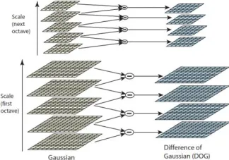
The main idea in SIFT consists of finding key points or interesting points which are invariant to scaling, rotation and illumination. For this aim, in the first step, a scale space for the processed image is constructed; It means that the original image is taken then progressively blurred out images are generated from it. Then, the original image is resized to half size, blurred out images are generated again and this process kept repeating itself. Mathematically, a blurred out image is generated by

convolving the Gaussian operator to the image pixels:

𝐿(𝑥, 𝑦; 𝜎) = 𝐺(𝑥, 𝑦, 𝜎) ∗ 𝐼(𝑥, 𝑦) (2)

where 𝐼(𝑥, 𝑦) and 𝐿 are the image and blurred image, respectively. 𝐺(𝑥, 𝑦, 𝜎) is the Gaussian operator. 𝑥, 𝑦 are local coordinates and 𝜎 is the scale parameter. The * denotes the convolution operation. The Gaussian operator is defined as follows:

𝐺(𝑥, 𝑦, 𝜎) =_2𝜋𝜎12𝑒−(𝑥

2_+𝑦2_{) 2𝜎⁄} 2

(3)

Figure 12 shows the scale space of a ball. The next step in SIFT algorithm is to calculate the Difference of Gaussians (DoGs). This is necessary to find out key points. The DoG is calculated from the difference of two consecutive scales as follows [16]:

𝐷(𝑥, 𝑦; 𝜎) = (𝐺(𝑥, 𝑦, 𝑘𝜎) − 𝐺(𝑥, 𝑦, 𝜎)) ∗ 𝐼(𝑥, 𝑦) =

𝐿(𝑥, 𝑦, 𝑘𝜎) − 𝐿(𝑥, 𝑦, 𝜎) (4)

Figure 13 shows a graphical representation for calculating DoGs.

The third step is to find the key points of the image. To find key points, in first instance, the approximate local maxima/ minima must be located in DoG images. To find these approximate local extrema, each pixel must be compared with its 26 neighbors (Figure 14).

A pixel is marked as a "key point" if it is the greatest or least of all its 26 neighbors. Usually, the extrema is laid between pixels and don’t match exactly on a pixel. In this case, the extremas are only "approximate" and a subpixel extrema search has to be performed mathematically.

Figure 12. Scale space of a ball with first and second octaves

Figure 13. Calculating the difference of Gaussians using

Using Taylor expansion of 𝐷(𝑥, 𝑦; 𝜎), the subpixel extrema is calculated as follows [16]:

𝒙̂ = − (𝜕_𝜕𝒙2𝐷𝟐)

−1𝜕𝐷

𝜕𝒙 (5)

where 𝒙 = [𝑥, 𝑦; 𝜎]𝑇and the derivatives of D are calculated at the last approximate extrema. Using the subpixel extrema as key points instead of approximat e extrema will increase the odds of matching and the stability of the SIFT algorithm.

A numerous quantity of key points may be obtained, some without enough contrast and some others lying along an edge. These key points are not useful in feature detections and must be omitted. To remove edge key points, Harris corner detector [17] can be used and for low contrast features, checking the key point intensity is a simple and useful way.

At this step, a set of key points is exploited with their scales. The scale of each key point is identical to the scale of its corresponding blurred image, making them s cale invariant. The fourth step of SIFT algorithm is to assign an orientation measure to each key point to provide orientation invariance.

To assign an orientation to a key point, the gradient magnitude and orientation of all pixels around the key point are calculated as follows:

𝑚(𝑥, 𝑦)

= √(𝐿(𝑥 + 1, 𝑦) − 𝐿(𝑥 − 1, 𝑦))2+ (𝐿(𝑥, 𝑦 + 1) − 𝐿(𝑥, 𝑦 − 1))2

𝜃(𝑥, 𝑦) =

tan−1((𝐿 (𝑥, 𝑦 + 1) − 𝐿(𝑥, 𝑦 − 1)) (𝐿 (𝑥 + 1, 𝑦) − 𝐿(𝑥 − 1, 𝑦))⁄ )

(6)

Then a histogram with 36 bins (each 10 degrees) is created using these magnitudes and orientations. The amount of histogram is proportional to the magnitude. The created histogram will have a peak at some points. The corresponding bin indicates the orientation assignable to the key point. Now, the objective of orientation invariance is also reached.

The final step in SIFT algorithm is to create a descriptor for each detected feature or key point. For this purpose, a 16*16 grid, partitioned into 4*4 windows , is considered around each key point (Figure 15). The gradient magnitudes and orientations are calculated within each 4*4 window.

Figure 14. The neighbors of a pixel in DoGs [16]

Based on the orientation-measure results, an 8-bin histogram is created. For the sake of accuracy, the magnitude in each bin can also be considered depending on the distance from the key point. So a more remote pixel from the key point will have a lesser contribution to the histogram. Applying this for the sixteen 4*4 windows, an array of 4*4*8 number is created for each key point. Normalizing this array, the feature vector or the feature descriptor is created. For more details such as practical details, corrections and theoretical details, please refer to literature [16].

Now, everything is ready to merge the two maps. Algorithm 3 shows the map merging steps using SIFT.

𝐀𝐥𝐠𝐨𝐫𝐢𝐭𝐡𝐦 𝟑 𝑀𝑎𝑝 𝑀𝑒𝑟𝑔𝑖𝑛𝑔 𝑢𝑠𝑖𝑛𝑔 𝑆𝐼𝐹𝑇

1: 𝐩𝐫𝐨𝐜𝐞𝐝𝐮𝐫𝐞 𝑀𝑒𝑟𝑔𝑒(𝑚𝑎𝑝(1), 𝑚𝑎𝑝(2)₎

2: 𝑰𝒎𝒂𝒈𝒆(𝟏)= 𝑐𝑜𝑛𝑣𝑒𝑟𝑡_𝑡𝑜_𝑖𝑚𝑎𝑔𝑒 (𝑚𝑎𝑝(1))

3: 𝑰𝒎𝒂𝒈𝒆(𝟐)= 𝑐𝑜𝑛𝑣𝑒𝑟𝑡_𝑡𝑜_𝑖𝑚𝑎𝑔𝑒 (𝑚𝑎𝑝(2))

4: [𝒌𝒆𝒚𝒑𝒐𝒊𝒏𝒕𝒔

(𝟏)_{, 𝒅𝒆𝒔𝒄𝒓𝒊𝒑𝒕𝒐𝒓𝒔}(𝟏)_]

= 𝑆𝐼𝐹𝑇(𝑰𝒎𝒂𝒈𝒆(𝟏))

5: [𝒌𝒆𝒚𝒑𝒐𝒊𝒏𝒕𝒔

(𝟐)_{, 𝒅𝒆𝒔𝒄𝒓𝒊𝒑𝒕𝒐𝒓𝒔}(𝟐)_]

= 𝑆𝐼𝐹𝑇(𝑰𝒎𝒂𝒈𝒆(𝟐))

6: 𝒎𝒂𝒕𝒄𝒉𝒆𝒅_𝒇𝒆𝒂𝒕𝒖𝒓𝒆𝒔

= 𝑚𝑎𝑡𝑐ℎ(𝒅𝒆𝒔𝒄𝒓𝒊𝒑𝒕𝒐𝒓𝒔(𝟏), 𝒅𝒆𝒔𝒄𝒓𝒊𝒑𝒕𝒐𝒓𝒔(𝟐)₎

7: 𝑯𝒐𝒎𝒐𝒈𝒓𝒂𝒑𝒉𝒚 𝒎𝒂𝒕𝒓𝒊𝒙

= 𝑅𝐴𝑁𝑆𝐴𝐶(𝒎𝒂𝒕𝒄𝒉𝒆𝒅_𝒇𝒆𝒂𝒕𝒖𝒓𝒆𝒔)

8: 𝑭𝒊𝒏𝒂𝒍 𝑴𝒂𝒑_{= 𝑡𝑟𝑎𝑛𝑓𝑜𝑟𝑚(𝑚𝑎𝑝}(1)_{, 𝑚𝑎𝑝}(2)_{, 𝑯𝒐𝒎𝒐𝒈𝒓𝒂𝒑𝒉𝒚 𝒎𝒂𝒕𝒓𝒊𝒙)}

9: 𝐞𝐧𝐝 𝐩𝐫𝐨𝐜𝐞𝐝𝐮𝐫𝐞

Merging algorithm, described here, consists of five steps. First, the robot-produced local maps are stored as images. In the next step, the features of the images are detected and their descriptors are computed. In the third step, the descriptors are matched with each other between two images. Feature matching is actually a straightforward process. The first feature from the first image is selected and the distances of its descriptor to all feature descriptors of the second image are computed. A matched feature in the second image has the smallest “distance” to the selected feature. This process is repeated for all features of the first image. David Lowe's ratio test can optionally be used for features matching [16]. Generally, only three pairs of matched features are needed to compute a transformation or homography matrix between two images.

Figure 15. Selection of pixels around a key point for

With more than three pairs, RANSAC algorithm [18] can be used for computing the homography matrix. Homography matrix computation is the fourth step of the merging algorithm. In the fifth step, the transformation calculated from the homography matrix is applied to images or maps and the two maps are then merged accordingly.

The proposed algorithm is executed for merging the maps obtained in the experiment phase (Figure 8 and Figure 9). The common key points of these two maps are shown in Figure 16. As one can see, the proposed algorithm could find the correct common features between two maps. After forming the homography matrix, the two maps are merged together. The result is shown in Figure 17. Comparing Figure 17 and Figure 7 shows that the local maps have been merged correctly. The time expended to merge the maps is about 20 seconds which is about 20% of the time consumed using R-map merging algorithm.

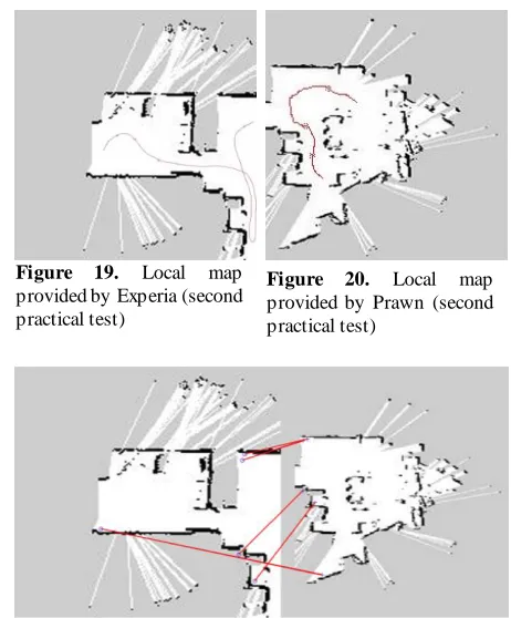
A second experiment is performed to map a more complex environment. This experiment is performed within a 50 𝑚2 location consisting of two compartments. The complete environment is shown in Figure 18. The local maps provided by Experia and Prawn are shown in Figures 19 and 20, respectively. Similar to the first practical test, the robots were conducted to explore their respective neighborhood manually and terminated their mission by checking a common landmark which was introduced earlier to them.

The matched points and the final merged map are also shown in Figures 21 and 22. As can be seen, the matched points have been found correctly and the merging process is well done.

Figure 16. Key points matching using the proposed merging

algorithm (first test)

Figure 17. The final merged map obtained by using the

proposed merging algorithm (first test)

Figure 18. 2D M ap of the environment considered for the

second practical test

Figure 19. Local map

provided by Experia (second practical test)

Figure 20. Local map

provided by Prawn (second practical test)

Figure 21. Key points matching using the proposed merging

algorithm (second test)

Figure 22. The final merged map using the proposed

3. CONCLUSION

In this paper, the map-merging algorithm using the maxima l empty rectangles (MER) concept is presented and implemented. It is shown here that this strategy is not only time-consuming, but also failed in the case of low overlap area.

To overcome these two inconveniences, an image feature extraction algorithm named SIFT is employed and a fast and reliable map-merging algorithm is proposed. Using SIFT, the local maps provided by ground robots are converted into images, and the features of each image together with their descriptors get extracted. These features are made invariant to orientation and scaling. Then, the matching features between the two images are identified and a homography matrix is finally computed using RANSAC.

Experimental results show the proposed map-merging algorithm can merge maps with the least common areas. Also, the proposed algorithm is meaningfully faster than the map-merging algorithm applying R-maps.

4. ACKNOWLEDGEMENT

We would also like to express our gratitude to Advanced Mechatronics and Robotics Laboratory (ARMLAB), Mechanical Engineering Department, Isfahan University of Technology for their generous contribution in preparing the facilities and the environment required.

5. REFERENCES

1. Rone, W. and Ben-Tzvi, P., “Mapping, localization and motion planning in mobile multi-robotic systems,” Robotica, Vol. 31, No. 1, (2013), 1–23.

2. Fenwick, J. W., Newman, P. M., and Leonard, J. J., "Cooperative concurrent mapping and localization", in 2002 IEEE

International Conference on Robotics and Automation, (2002),

1810–1817.

3. Konolige, K., Fox, D., Ortiz, C., Agno, A., Eriksen, M., Limketkai, B., Ko, J., Morisset, B., Schulz, D., Stewart, B., and Vincent, R., “Centibots: Very large scale distributed robotic teams,” Springer Tracts in Advanced Robotics, Vol. 21, No. 1, (2006), 131–140.

4. T hrun, S., “A Probabilistic On-Line Mapping Algorithm for T eams of Mobile Robots,” The International Journal of Robotics Research, Vol. 20, No. 5, (2001), 335–363. 5. Williams, S. B., Dissanayake, G., and Durrant -Whyte, H.,

"T owards multi-vehicle simultaneous localisation and mapping",

in Proceedings 2002 IEEE International Conference on Robotics

and Autom ation, Vol. 3, 2743–2748, (2002).

6. T hrun, S. and Liu, Y., “Multi-robot SLAM with sparse extended information filers,” Robotics Research, Vol. 15, No. 1, (2005), 254–266.

7. Carpin, S., Birk, A., and Jucikas, V., “On Map Merging,”

International Journal of Robotics and Autonomous Systems, Vol. 53, No. 1, (2005), 1–14.

8. Birk, A. and Carpin, S., "Merging Occupancy Grid Maps From Multiple Robots", in Proceedings of the IEEE, Vol. 94, No. 7, 1384–1397, (2006).

9. Saeedi, S., Paull, L., Trentini, M., and Li, H., “Neural Network-Based Multiple Robot Simultaneous Localization and Mapping,”

IEEE Transactions on Neural Networks, Vol. 22, No. 12, (2011), 2376–2387.

10. Saeedi, S., Paull, L., T rentini, M., Seto, M., and Li, H., "Efficient map merging using a probabilistic generalized Voronoi diagram",

in 2012 IEEE/RSJ International Conference on Intelligent Robots

and System s, 4419–4424, (2012).

11. Dinnissen, P., Givigi, S. N., and Schwartz, H. M., "Map merging of Multi-Robot SLAM using Reinforcement Learning", in 2012 IEEE International Conference on System s, Man, and

Cybernetics (SMC), 53–60, (2012).

12. Li, H., T sukada, M., Nashashibi, F., and Parent, M., “Multivehicle cooperative local mapping: A methodology based on occupancy grid map merging,” IEEE Transactions on Intelligent Transportation Systems, Vol. 15, No. 5, (2014), 2089–2100. 13. Park, J., Sinclair, A. J., Sherrill, R. E., Doucette, E. A., and Curtis, J. W., "Map merging of rotated, corrupted, and different scale maps using rectangular features", in 2016 IEEE/ION Position,

Location and Navigation Symposium (PLANS), 535–543, (2016).

14. Park, J., "A Reduced Element Map Representation and Applications: Map Merging, Path Planning, and T arget Interception". PhD T hesis: Aerospace Engineering, Auburn University, (2017).

15. Ahn, J. G. and Jeon, H. S., "R-Map : A Hybrid Map Created by Maximal Rectangles", in ICCAS 2010, 1336–1339, (2010).

16. Lowe, D. G., “ Distinctive image features from scale-invariant keypoints,” International journal of computer vision, Vol. 60, No. 2, (2004), 91–110.

17. Harris, C. and Stephens, M., "A combined corner and edge detector.", in Proceedings of Fourth Alvey vision conference, Vol. 15, No. 50, 147–151, (1988).

Map-merging in Multi-robot Simultaneous Localization and Mapping Process Using

Two Heterogeneous Ground Robots

S. Hadian Jazi, S. Farahani, H. Karimpour

Department of Mechanical Engineering, University of Isfahan, Iran

P A P E R I N F O

Paper history: Received 16 October 2018

Received in revised form 05 March 2019 Accepted 07 March 2019

Keywords: Map-merging

Multi-agents Simultaneous Localization and Mapping

Ground Robot Image Processing

هدیکچ

هسورپ کی رد و یلخاد طیحم کی زا یلک هشقن دیلوت یارب دامتعا لباق و عیرس هشقن بیکرت متیروگلآ کی هلاقم نیا رد هشقن هدش هئارا یتابر دنچ نامزمه تیعقوم نییعت و یرادرب ریسم ندرک ادیپ و طیحم کی رد تکرح یارب تابر کی .تسا

تکرح هشقن هب دوخ .تسا هتسباو طیحم نآ رد دوخ تیعقوم هب طیحم زا هشقن هیهت یارب نینچمه و دراد زاین طیحم زا یا

هشقن ار هدیچی هلاسم نیا یم نامزمه تیعقوم نییعت و یرادرب

طیحم رد .دنیوگ لمج زا یتوافتم لیلاد هب ،هدیچیپ و گرزب یاه

ه

ینلاوط و اطخ یگتشابنا دافتسا ،هسورپ ندش

هشقن یارب تابر کی زا ه هیجوت یرادرب

زا لاومعم دراوم نیا رد .تسین ریذپ دنچ

یم هدافتسا راک نیا یارب تابر هسورپ رد اهشلاچ نیرتمهم زا یکی .دوش

هشقن یتابردنچ یاه بیکرت ،یرادرب

ن ندرک هشق یاه

هیهت یلحم یلک هشقن دیلوت سپس و نآ زا یشخب ای و طیحم زا تابر ره طسوت هدش وگلآ کی هلاقم نیا رد .تسا طیحم نآ

متیر

یگژیو هیاپ رب هشقن بیکرت یارب یزکرم هصخشم و اه

هشقن یاه یم هئارا یلحم یاه لیبق زا یتاعلاطا هب نآ رد هک دوش

تابر یبسن تیعقوم ای هیلوا تیعقوم هب .تسین یزاین اه

هب متیروگلآ نیا یبایشزرا روظنم توافتم تابر ود زا یبرجت تروص

دنتسه زهجم طیحم شیوپ یارب یتوافتم یرزیل یاهروسنس هب هک یم

دوش یم ناشن شیامزآ جیاتن . متیروگلآ هک دهد

یفرعم هدش

بیکرت یارب یبسانم تعرس و تقد هشقن ندرک

دراد طیحم زا یلک هشقن دیلوت و یلحم یاه .