Finite sample criteria for autoregressive model order selection

© Shiraz University

FINITE SAMPLE CRITERIA FOR AUTOREGRESSIVE

MODEL ORDER SELECTION*

M. KARIMI**

Dept. of Electrical Engineering, School of Engineering, Shiraz University, Shiraz, I. R. of Iran Email: karimi@shirazu.ac.ir

Abstract– The existing theoretically derived order selection criteria for autoregressive (AR) processes have poor performance in the finite sample case. In this paper, the least-squares-forward (LSF) is considered as the AR parameter estimation method, and new theoretical approximations are derived for the expectations of residual variance and prediction error. These approximations are especially useful in the finite sample case and are derived for AR processes with arbitrary statistical distributions. New order selection criteria for AR processes are derived using these approximations. In a simulation study, the performance of the proposed criteria relative to other criteria is examined in the finite sample case. Simulation results show that the performance of the proposed criteria is much better than the other theoretically derived criteria.

Keywords– Autoregressive process, AR model, order selection, information criterion, residual variance, prediction error

1. INTRODUCTION

An important step in AR modeling is the selection of the model order. An order selection criterion is usually used to determine the appropriate order for the AR model. In the past four decades, the AR order selection problem has been the subject of many researches. Results of some of the recent works on this problem can be seen in [1-11].

Two different cases can be distinguished in the AR model order selection. The first is the large sample (or asymptotic) case in which the number of given data (N) is large compared to the maximum candidate order. The second is the finite sample case in which N is not large compared to the maximum candidate order. Many of the existing order selection criteria are developed based on the asymptotic theories, and hence, are more useful in the large sample case. It is well known that these asymptotic criteria can be quite biased in the finite sample case.

The first asymptotic criteria to gain widespread acceptance were the Akaike's final prediction error (FPE) criterion [12] and the Akaike information criterion (AIC) [13]. FPE gives an estimate of the prediction error. "Prediction error" means the one-step prediction mean squared error for a realization of the process independent of the one observed. AIC was designed to be an approximately unbiased estimator of the Kullback-Leibler index of the fitted model relative to the true model. Hurvich and Tsai [14] proposed a corrected version of AIC, denoted AICC, which is less biased in the finite sample case. Cavanaugh [15] introduced the Kullback information criterion (KIC) as an asymptotically unbiased estimate of Kullback's symmetric divergence. As for AIC, KIC is strongly biased in the finite sample case. Recently, Seghouane and Bekara [16] proposed KICC, which is an approximately unbiased correction of KIC in the finite sample case.

The criteria FPE, AIC, AICC, KIC, and KICC are (asymptotically) efficient, but they are not consistent. An efficient order selection criterion chooses an AR model which achieves the optimal rate of convergence of the prediction error [17]. An order selection criterion is said to be consistent if it chooses the true order with probability one as N→∞. Consistency can be obtained only at the cost of efficiency. Usually, of the two properties, efficiency is preferred. Rissanen [18] developed the minimum description length (MDL) criterion which is consistent. Schwarz [19] introduced a similar consistent criterion based on Bayesian reasoning. Another consistent criterion has been developed by Hannan and Quinn [20].

Several AR order selection criteria, designed for the finite sample case, are introduced by Broersen and Wensink [21, 22]. The values of the parameters used in these criteria are given by empirical formulas. For each of the well-known AR estimation methods, Broersen and Wensink proposed a different empirical formula for these parameters. The first criterion is the finite sample criterion (FSC) [21], which gives an estimate of the prediction error. This criterion was designed to replace the FPE criterion in the finite sample case. Another criterion is the finite sample information criterion (FIC) [21]. It was designed to replace the generalized information criterion (GIC), which is the general form of the criteria like AIC and MDL, in the finite sample case. The third criterion is the finite sample information criterion (FSIC) [22], which is an estimator of the Kullback-Leibler index. For the case where the AR parameter estimation method is LSF (also known as the covariance method), Karimi [23] modified these three finite sample criteria and proposed the MFSC (modified FSC), MFIC, and MFSIC criteria. These modified criteria are obtained by introducing a new empirical formula for the parameters used in FSC, FIC, and FSIC, respectively. He showed that these modified criteria outperform the former criteria FPE, AIC, AICC, MDL, FSC, FIC, and FSIC, in the finite sample case.

In this paper, we will derive new approximations for the expectations of residual variance and prediction error in the case that the AR parameter estimation method is LSF. These approximations are derived using the theoretical descriptions given in [23] for the residual variance and prediction error of the LSF method. Based on these new approximations, new criteria are developed for AR model order selection. Simulation results show that, in the finite sample case, one of these criteria has the best performance among all existing order selection criteria which have a theoretical basis.

The remainder of this paper is organized as follows. In section 2, we briefly review the theoretical descriptions derived in [23] for the residual variance and the prediction error of the LSF method. In section 3, new approximations for the expectations of residual variance and prediction error are derived and these approximations are used for developing new order selection criteria. Using simulations, the performance of the proposed order selection criteria is evaluated and compared with the existing criteria in section 4.

2. THEORETICAL DESCRIPTIONS FOR THE RESIDUAL VARIANCE AND THE PREDICTION ERROR

A real AR(p) process is given by

) ( ) ( ... ) 2 ( ) 1 ( )

(n a₁x n a₂x n a x n p w n

x = − + − + + _p − + (1)

where

a

1

,

...

,

a

p are the real coefficients of the process and p is the process order. w(.) is a real

independent, identically distributed (i.i.d.) random process with zero mean and variance 2 w

σ . It is assumed that the AR model is stable. It follows from these assumptions that the process x(.) is zero mean, and in addition, it is mean and covariance ergodic.

) ( ˆ ) ( ˆ ... ) 2 ( ˆ ) 1 ( ˆ )

(n a₁x n a₂x n a x n q w n

x = − + − + + _q − + (2)

In the remainder of this paper, we will always assume that the AR estimation method is LSF. Residual variance, which is a measure of the fitness of the above model to the given data, is defined as follows:

∑

∑

+ = = ∧ − − − = N q i q j

jxi j a i x q N q S 1 2 1

2_{( )} 1 _{[ () ( )] (3)}

Prediction error is a measure of the fitness of the estimated model (given by (2)) to the samples of a realization of the AR process independent of the observed one. It is defined as

      − − =       − − − =       − − − =

∑

∑

∑

∑

∑

= ∧ + = = ∧ + = = ∧ 2 1 1 2 1 1 2 1 ] ) ( ) ( [ ] ) ( ) ( [ 1 ] ) ( ) ( [ 1 ) ( q j j y N q i q j j y N q i q j j y j i y a i y E j i y a i y E q N j i y a i y q N E q PE (4)

where y(i)’s are samples of any other realization of the AR process, and E_y{.} is the expectation operator over these realizations.

For the AR process given by (1), let us define the random variables z(n,i) as follows:

1 ; ]} )) , ( ) ( [( { ) , ( ) ( 1 ; ) 1 ( ) , ( 5 . 0 2        > − − − − = − = ∧ ∧ i i n x i n x E i n x i n x i n x i n z MS MS x

σ

(5)

where

σ

_x is the standard deviation of x(.), and x_MS∧ (n,i) is the linear minimum mean square error (LMMSE) estimate of x(n-i) given z(n,1), z(n,2), … , and z(n,i-1). The random variables z(n,i) are results of a Gram-Schmidt orthogonalization process. Thus, it is obvious that xMS(n,i)

∧

is also the LMMSE estimate of x(n-i) given x(n-1), x(n-2), … , and x(n-i+1). It can easily be seen that

, 0 , 0 ; 0 )] , ( ) , (

[z n i z n j i j i j

E = ∀ > ∀ > ≠ (6)

_E[_z2(_n,_i)]₌1 ;_∀i>0 ₍₇₎ Now we define

Z=[z₁,z₂,...,z_q] (8) Where q i i N z i q z i q

z_{( 1, ) ( 2, ) ... ( , )]}T _{; 1,2,...,}

[ + + =

= i

z (9)

It can be shown that for any order q greater than or equal to the true order p [23]

p q i c q PE q i w

w+ = + ≥

=

∑

= ∧ ∧ ∧ ; ) ( ) ( 1 2 2 2

σ

σ

c c

T (10) and thus p q i c E E q PE E q i w

w+ = + ≥

=

∑

= ∧ ∧ ∧ ; ] ) ( [ ] [ )] ( [ 1 2 2 2

σ

σ

c c

T

(11)

1 q T 1

T_{Z Z w}

Z

c − +

∧

=( ) (12) where

T N w q

w q

w( 1) ( 2) ... ( )]

[ + +

=

+1 q

w (13)

In addition, the following description can be derived for the expectation of residual variance [23]

p q E

q N q

S

E _w ≥

− −

= 1 [∧ ∧] ;

)] (

[ 2

σ

2 _cT_ZT_{Zc (14)}

In the case where N−q>>1, it can be shown that [23]

)

( _q

T_{Z I}

Z ≈ N−q (15)

where I_q is the q by q identity matrix. Substituting (15) in (14), we obtain

p q i

c E E

q S E

q

i w

w− = − ≥

≈

∑

= ∧ ∧

∧

; ] ) ( [ ]

[ )]

( [

1

2 2

2

2

σ

_{c c}

σ

T

(16)

In the next section, we will use (11) and (16) to derive new approximations for the expectations of prediction error and residual variance.

3. DERIVATION OF THE NEW ORDER SELECTION CRITERIA a) Statistical properties of the c(∧i)

In the previous section we saw that the elements of the vector c∧ have a key role in the descriptions given for PE(q) and _S2(_q)_{. Thus, it is important to determine the statistical properties of these elements. One of} these properties will be used in deriving new approximations for residual variance and prediction error and proposing a new estimate for the prediction error. The other properties are also useful because they may be used for determining the statistical properties of the prediction error and the residual variance. In addition, they may be used for deriving better estimates for the prediction error in the future.

In the remainder of this paper we will assume that N−q>>1. As discussed in [23], this assumption is not in conflict with the finite sample assumption in nearly all cases. So, the results that we obtain in this paper can be used in both large sample and finite sample cases.

Substituting (15) in (12), we obtain

1

1 q T_w

Z

c +

∧

− ≈

q

N (17) and thus

∑

−

= +

∧

+ +

− = −

≈ N q

k

i k q z k q w q N q

N i c

1

) , ( ) ( 1

1 )

( T _{q 1}

i w

z (18)

Each random variable z(n,i) is a linear combination of x(n-1), x(n-2), … , and x(n-i). On the other hand,

w(n) is independent of x(n-i) for each i>0. Therefore, w(n) is independent of z(n,i). So, we can obtain the mean of the c(∧i) as follows:

0 )] , ( [ )] ( [ 1

)] , ( ) ( [ 1

] ) ( [

1 1

= + +

− = + +

−

≈

∑

∑

−

= −

=

∧ N q

k q

N

k

i k q z E k q w E q N i k q z k q w E q N i c

where we have used the fact that w(.) is a zero mean process. Using (18), we can write

] [ ) ( 1 )] , ( ) ( ) , ( ) ( [ ) ( 1 ] ) ( [ 1 1 , , 2 1 1 2 2

∑ ∑

∑ ∑

− = − = − = − = ∧ − = + + + + − ≈ q N k q N s i s k q N k q N s b E q N i s q z s q w i k q z k q w E q N i c E (20)

where b_k,_s,_i is defined as follows:

) , ( ) ( ) , ( ) ( ,

, w q k z q k i w q s z q si

b_ksi = + + + + (21)

Now, we want to determine the expectation of b_k,s,i. We know that z(n,i) is a linear combination of x(n-1), x(n-2), … , and x(n-i). Thus, it is obvious that w(m) is independent of z(n,i) for m≥n and i>0. If k>s, then

q+k>q+s and w(q+k) will be independent of w(q+s). It can be seen from these properties that if k>s, then

w(q+k) will be independent of the other three variables in the right hand side of (21). It follows that

s

k

i

s

q

z

s

q

w

i

k

q

z

E

k

q

w

E

b

E

[

_k,s,i

]

=

[

(

+

)]

[

(

+

,

)

(

+

)

(

+

,

)]

=

0

;

>

(22) It can be shown in a quite similar way that, if k<s, then w(q+s) will be independent of the other three variables in the right hand side of (21). It follows that

;

0

)]

,

(

)

(

)

,

(

[

)]

(

[

]

[

b

_{, ,}

E

w

q

s

E

z

q

k

i

w

q

k

z

q

s

i

k

s

E

_ksi

=

+

+

+

+

=

<

(23)

We know that w(q+k) is independent of z(q+k,i). Thus, it follows from (7) that

; )] , ( [ )] ( [ )] , ( ) ( [ ]

[ 2 2 2 2 2

,

, E w q k z q k i E w q k E z q k i k s b

E _ksi = + + = + + =

σ

_w = (24)

Substituting (22), (23), and (24) in (20), we obtain

2 1 2 2 2 ₁ ) ( 1 ] ) ( [ w q N k w q N q N i c

E

σ

σ

− = − ≈

∑

− = ∧ (25)

Another statistical property of the elements of c∧ is the correlation between these elements. It is shown in the appendix that these elements are approximately uncorrelated, i.e.

; 0 ] ) ( ) (

[ci c j i j

E ∧ ∧ ≈ ≠ (26)

Note that in deriving the statistical properties of c(∧i)'s we have not assumed a particular probability density function (pdf) for the w(.) process and the properties obtained are valid for any pdf. Thus, the results that we will obtain based on these properties will be valid for any pdf as well.

b) The FPEF criterion

Substituting (25) in (11) and (16), we obtain

p q q N q q N q PE

E q _w

i

w

w+ ₋ = + ₋ ≥

≈

∑

= ; ) (1 1 )] ( [ 2 1 2

2

σ

σ

σ

(27)

p q q N q q N q S E _w q i w

w− ₋ = − ₋ ≥

≈

∑

= ; ) (1 1 )] ( [ 2 1 2 2

These new theoretical approximations for the expectations of the prediction error and the residual variance are very important and enable us to derive new order selection criteria. Note that the expressions given in (27) and (28) do not depend on the true process order p. This shows that the behavior of the expectations of PE(q) and _S2(_q) _{is (approximately) independent of the true process order if q is greater than or equal} to the true process order. It is worth noting that the relations (15)-(20) and (26)-(28) become exact in the case that (N−q)→∞.

It follows from (27) and (28) that

;

2 1

1

)] ( [

)] ( [

2 _{N q} q p

N

q N

q q N

q

q S E

q PE

E _≥

− =

− −

− +

≈ (29)

Therefore, we can use the following expression for estimating the prediction error for each order q

p q q

N N q S q S q S E

q PE E q

PE ≥

− =

=

∧

; ) 2 )( ( ) ( )] ( [

)] ( [ )

( 2 2

2 (30)

It is reasonable to choose the integer q that minimizes this estimate as the appropriate order for the autoregressive process. Thus, we propose the finite sample FPE (FPEF) criterion as follows:

) 2 )( ( )

( 2

q N

N q S q FPEF

−

= (31)

The FPE criterion is defined as follows [12]:

) )( ( )

( 2

q N

q N q S q FPE

− +

= (32)

It is an estimate of the prediction error in the asymptotic case (N→∞). In the finite sample case, this estimate is negatively biased and this bias can be quite large. This bias often leads to overestimation in the finite sample case.

We can rewrite FPE and FPEF in the following way:

  

 

  

 

− + =

N q N q q S q FPE

1 1 ) ( )

( 2

(33)

   

 

   

 

− −

− + =

q N

q q N

q

q S q FPEF

1 1 ) ( )

( 2

(34)

Thus, the term

(

q N

)

in FPE(q) is replaced by the term

(

q

(

N−q

)

)

in FPEF(q). For each q, the term

(

)

(

q N−q

)

is greater than

(

q N

)

. Thus, it can easily be seen from (33) and (34) that for each q, the estimate that FPEF(q) gives for the prediction error is greater than FPE(q). Moreover, as q increases, the growth of

(

q

(

N−q

)

)

is more rapid than

(

q N

)

. Therefore, as q increases, the difference between FPEF(q) and FPE(q) increases as well. Especially, it can be seen from (31) and (32) that, as q approaches

simulations to show the less bias and better performance of FPEF in estimating the prediction error in the finite sample case. It can easily be seen from (33) and (34) that, in the asymptotic case, the two criteria become identical.

An empirical criterion for AR model order selection is the FSC criterion defined as [21]

1 1 ) ( ) ( 1 2

∏

=      − + = q i i i v v q S q

FSC (35)

where the v_i's are given by the following expression when the LSF method is used for parameter estimation 2 2 1 + − = i N

vi (36)

FSC gives an estimate of the prediction error and it was designed to replace FPE in the finite sample case. In order to compare FPEF and FSC, it is better to derive alternative expressions for these criteria. It can be seen from (36) that

) 1 )( 2 1 ( ... ) 4 2 5 2 )( 2 2 3 2 ( ) 1 ( 1 N N N N q N q N q N q N v q i i + − − + − + − + − + − = +

∏

= (37) ) 1 )( 2 3 ( ... ) 4 2 3 2 )( 2 2 1 2 ( ) 1 ( 1 N N N N q N q N q N q N v q i i − − − + − + − + − + − = −

∏

= (38)

Combining (37) and (38), we get

1 2 1 1) -3)(N -(N ... ) 3 2 )( 1 2 ( 1) 1)(N -(N ... ) 5 2 )( 3 2 ( 1 1

1 − +

+ = + − + − + + − + − =       − +

∏

= N q

N q N q N q N q N v v q i i

i ₍₃₉₎

Substituting (39) in (35), we obtain

) 1 2 1 )( ( ) ( 2 + − + = q N N q S q

FSC (40)

On the other hand, we can derive an expression similar to (35) for FPEF, i.e.

1 1 ) ( ) ( 1 2

∏

=      − + = q i i i w w q S q

FPEF (41)

where w_i's are defined by the following relation:

2 2 2 ) 1 ( 2 2 ) 1 ( ) 1 ( ) ( ) ( 1 1 2

2 _{N i}

i N i N N i N N i S i FPEF i S i FPEF w w i i − + − = − − − =       − −       = − + (42)

Solving (42) for wi, we get

1 2 1 + − = i N

w_i (43)

that the performance of FPEF in estimating the prediction error is better than that of FSC. Similar results can be obtained by comparing (31) and (40). It can be seen from these relations that the two criteria FSC and FPEF have similar expressions. In addition, it can easily be seen that, the estimate which FPEF gives for the prediction error can be much greater than that of FSC for q near (N/2). It can also be seen from (31) and (40) that the two criteria are identical in the asymptotic case.

As we saw, w_i is always greater than v_i. Thus, )

) 1 (

) ( )( 1 1 ( ) 1 (

) (

2 2

− −

+ =

− S q

q S w w q

FPEF q FPEF

q

q _{is always greater}

than )

) 1 (

) ( )( 1 1 ( ) 1 (

) (

2 2

− −

+ =

− S q

q S v v q

FSC q FSC

q

q _{. That is, for all q, FPEF(q) has a more rapid increase with q than}

FSC(q). This shows that the overfit probability of FPEF is always less than that of FSC. It can be shown in a similar way that, for all q>1, FPEF(q) has a more rapid increase with q than FPE(q). Thus, the overfit

probability of FPEF is less than that of FPE in nearly all cases. Simulation results given in the next section are in agreement with these explanations.

Recently, a new empirical formula is proposed for the parameters v_i in FSC. This new formula is [23].

] ) ( 5 . 1 1 )[ 6 . 1 2 (

1

2 N

i i

N vi

− +

−

= (44)

The criterion which is obtained by using this formula for v_i's in (35) is named as modified FSC (MFSC) [23]. The performance of MFSC in estimating the prediction error will also be evaluated and compared with those of FPE, FSC, and FPEF in section 4.

As we saw, the empirical formula for parameters of FSC can be replaced by (43), which is a theoretical formula. The parameters of FSC are also used in FIC which is another empirical criterion for AR model order selection. Thus, it is possible to use the formula given by (43) for parameters of FIC as well. FIC is defined as follows [21]:

)]

( ln[ ) , (

1

2

∑

=

+

= q

i i v q

S q

FIC

α

α

(45)

where v_i's are given by (36). FIC was proposed to replace GIC in the finite sample case. GIC is defined as follows:

N q q S q

GIC( ,

α

)=ln[ 2( )]+

α

₍₄₆₎

GIC is a general form for several order selection criteria. For example, by substituting α=2 and )

ln(N

=

α in GIC, AIC and MDL criteria are obtained, respectively. Using the formula given by (43) for parameters of FIC, we obtain the FICA criterion

∑

=

+

= q

i i w q

S q

FICA

1 2_{( )]}

ln[ ) ,

(

α

α

(47)

Like FIC, FICA is an empirical criterion because it is obtained by changing the formula for the parameters of FIC and it has not been derived theoretically. Another modification for FIC can be obtained by using the formula given by (44) for its parameters [23]. This criterion is named modified FIC (MFIC) [23].

c) The AICF criterion

(

)

[

]

{

θ

}

θ

θ| ) _θ 2ln (1 ) ,... , ( ) ;ˆ

( =E − f y y N

∆ ∧ (48)

where θ and θˆ are the vectors containing the parameters of the true and fitted AR models respectively

T q w

T q

wa a ...a ] , ˆ [ˆ aˆ aˆ ...aˆ ]

[ 2 _{1 2}

2 1

2

σ

σ

=

= θ

θ (49)

where

ˆ 1 [ () ( )] 2( )

1

2

1

2 _{xi a xi j S q}

q N N q i q j j

w = ₋

∑

−

∑

− =

+

= =

∧

σ

(50)

θ

E denotes the expectation under the true model, and this expectation is taken assuming that θˆ is

deterministic. f(…) is the joint pdf of y(1) … y(N) under the fitted model. In this subsection, we assume that the AR process is Gaussian. Thus

(

)

∏

[

]

=              ₋ − = N

i _w w

i y i y N y y f 1 2 2

2 2ˆ

) ( ˆ ) ( exp ˆ 2 1 ˆ ; ) ( , ... , ) 1 (

σ

σ

π

θ (51)

where ) ( ˆ ) ( ˆ 1

∑

= − = q j

jyi j a

i

y (52)

It follows from (51) that

(

)

[

]

[

]

( )

∑

[

]

∑

= =       ₋ + + =      − _{− −} − − = − N i w w N i w w i y i y N N i y i y N y y f 1 2 2 2 1 2 2 2 ˆ ) ( ˆ ) ( ˆ ln ) 2 ln( ˆ 2 ) ( ˆ ) ( ) ˆ ln( 2 1 ) 2 ln( 2 1 2 ˆ ; ) ( , ... , ) 1 ( ln 2

σ

σ

π

σ

σ

π

θ (53)

Substituting (53) in (48) and using (4), (50) and (52), we obtain

( )

[

]

( )

{

[

]

}

( )

(

)

) ( ) ( ) ( ln ) 2 ln( ˆ ) ( ˆ ln ) 2 ln( ˆ ) ( ˆ ) ( ˆ ln ) 2 ln( ˆ ) ( ˆ ) ( ˆ ln ) 2 ln( ) | ( 2 2 1 2 2 1 2 2 2 1 2 2 2 q S q PE N q S N N q PE N N i y i y E N N i y i y E N N N i w w N i w y w N i w y w + + = + + = − + + =       ₋ + + = ∆

∑

∑

∑

= = = ∧

π

σ

σ

π

σ

σ

π

σ

σ

π

θ θ (54)

The prediction error cannot be computed and we substitute its estimate given by (30) in (54) to obtain an estimate of the Kullback-Leibler index as follows

2 )] ( ln[ ) 2 ln( ) | ( 2 2 q N N q S N N − + + ≈

∆

θ

∧

θ

π

(55)

q N

q q

S q

AICF

2 2 )] ( ln[ )

( 2

− +

= (56)

which can also be written as

1 -1

1 )]

( ln[ ) (

1 2

   

 

     

− + +

=

∏

= q

i i

i w w q

S q

AICF (57)

where w_i's are given by (43). The AIC criterion is defined as

N q q S q

AIC( )₌ln[ 2( )]₊2 ₍₅₈₎

It was designed to be an estimator of the Kullback-Leibler index in the asymptotic case. Thus, AIC can be replaced by AICF in the finite sample case. It can be seen that AICF approaches AIC as N→∞. Another corrected version of AIC is AICC which is defined as [14]

2 2 2 )] ( ln[ )

( 2

− −

+ + =

q N

q q

S q

AICC (59)

It was proposed to modify the performance of AIC in the finite sample case.

We should note here that if we substitute the estimate which FPE gives for PE(q) in (54), we can obtain the following criterion for AR order selection in the same way that we obtained AICF

q N

q q

S

− + 2

)] ( ln[ 2

It can be seen that this criterion is close to AICC.

Broersen and Wensink [22] replaced PE(q) in (54) by its empirical estimate given by

∏

= −

+ q

i i

i

v v q

S

1

2 ₎

1 1 ( ) ( and derived the FSIC criterion in the same way that we derived AICF. Thus, the FSIC is defined as

1 1

1 )]

( ln[ ) (

1

2 ₋

   

 

     

− + +

=

∏

= q

i i

i v v q

S q

FSIC (60)

where vi's are given by (36). Using (39), it can also be written as

1 2 2 )] ( ln[ )

( 2

+ − + =

q N

q q

S q

FSIC (61)

Another criterion can be derived by using the empirical formula given by (44) for the parameters v_i

in (60). This criterion is named MFSIC [23]. It can easily be seen that, in the asymptotic case, the criteria MFSIC, FSIC, AICC, and AICF become identical with AIC. So, these four criteria are (asymptotically) efficient because AIC is efficient itself.

It can be seen from (56) and (61) that the expressions for AICF and FSIC are very similar. However, for values of q near (N/2), the difference between the penalty factors of these two criteria is significant. In the vicinity of (N/2), the penalty factor of AICF has a more rapid increase with q. It can also be seen that, in the vicinity of (N/2), the increase in the penalty factor of AICF with q is much more than the increase in the penalty factors of AIC and AICC, but less than the increase in the penalty factor of MFSIC. In section 4, we will use simulations to compare the performance of these criteria in AR model order selection.

4. SIMULATIONS

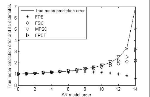
The first criterion proposed in this paper is FPEF. It gives an estimate of the prediction error for orders greater than or equal to the true process order. Thus, it is important to compare this estimate with the true prediction error and with the estimates that the criteria FPE, FSC, and MFSC give for the prediction error. We saw in the previous section that the behavior of the expectations of PE(q) and _S2(_q) _is (approximately) independent of the true process order if q is greater than or equal to the true process order. The simplest AR process is white noise (a zero order AR process). Thus, the behavior of the expectations of PE(q) and _S2(_q) _{for white noise is typical for all other processes above their true order. Therefore, we} compare the performance of the above-mentioned criteria in estimating the prediction error for the white noise process. Figures 1-3 show the performance of FPEF, FPE, FSC, and MFSC in estimating the prediction error when the number of observations N is equal to 12, 30, and 50, respectively. The results shown in each figure are obtained by averaging over 50000 independent simulation runs of N Gaussian white noise samples. The results given in these figures show that MFSC gives the best estimates for the prediction error. However, note that MFSC and FSC are empirical criteria and among the two theoretical criteria, the performance of FPEF is much better than FPE. In addition, the estimates that FPEF gives for the prediction error are better than those of FSC.

Fig. 1. Comparison of averages of the true prediction error, FPE, FSC, MFSC, and FPEF, for 50000 independent simulation runs of 12 samples of white Gaussian

noise. The AR parameter estimation method is LSF

Fig. 2. Comparison of averages of the true prediction error, FPE, FSC, MFSC, and FPEF, for 50000 independent simulation runs of 30 samples of white Gaussian

Fig. 3. Comparison of averages of the true prediction error, FPE, FSC, MFSC, and FPEF, for 50000 independent simulation runs of 50 samples of white Gaussian

noise. The AR parameter estimation method is LSF

The performance of the order selection criteria can be evaluated and compared by evaluating and comparing the quality of the AR models that they choose. A measure for quality of a model chosen for a given AR process is the model error (ME) which is defined as [24]

   



 − = ( )₂ 2

) (

w w q PE N q ME

σ

σ

(62)

where q is the selected model order. Model error (ME) is a normalized version of the prediction error after subtraction of 2

w

σ .

Tables 1 and 2 give comparisons of average ME for models selected by the criteria proposed in this paper and by the other existing criteria. These performance comparisons are made in the finite sample case. The criteria GIC, FIC, MFIC, and FICA with α=2 are omitted from the tables because their performances are close to the performances of FPE, FSC, MFSC, and FPEF, respectively. The KIC and AKICC criteria, whose performances are presented in these tables, are defined as follows [15, 16]:

N

q

q

S

q

KIC

(

)

=

ln[

2

(

)]

+

3

₍₆₃₎

)

(

)

2

(

)

2

3

)(

1

(

)]

(

ln[

)

(

2

q

N

N

q

q

N

N

q

N

q

q

S

q

AKICC

−

+

−

−

−

−

+

+

=

(64)

Note that AKICC is an approximation of KICC [16].

Table 1. Average model error ME with different order selection criteria for three Gaussian AR processes with orders 2, 3, 4, and reflection coefficients k_i =(0.2)i. N is equal to 14, and 0 and 6 are the minimum and maximum

candidate orders, respectively. Average ME values are obtained using 50000 independent simulation runs and the AR parameter estimation method is LSF

_____________________________________________________________________________________________ | α =ln(N) |

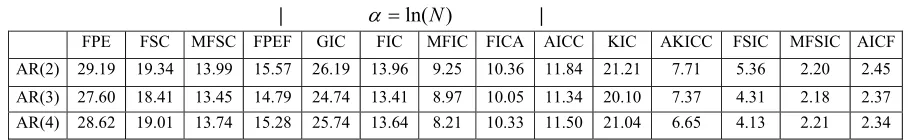
Table 2. Average model error ME with different order selection criteria for three Gaussian AR processes with orders 2, 3, 4, and reflection coefficients k_i =(−0.6)i. N is equal to 30, and 0 and 14 are the minimum

and maximum candidate orders, respectively. Average ME values are obtained using 50000 independent simulation runs and the AR parameter estimation method is LSF

_____________________________________________________________________________________

| α =ln(N) |

FPE FSC MFSC FPEF GIC FIC MFIC FICA AICC KIC AKICC FSIC MFSIC AICF AR(2) 169.02 86.40 47.61 67.23 141.58 27.64 10.96 16.41 104.54 153.40 77.21 4.97 4.53 4.64 AR(3) 181.47 97.82 55.16 75.18 154.72 32.34 13.73 20.18 115.32 165.29 90.08 6.20 5.68 5.81 AR(4) 183.26 96.83 54.83 77.36 158.52 30.08 12.38 18.99 116.48 168.00 89.40 6.62 6.10 6.23 In Table 3, we have considered the case that the process is actually an MA(1) process, but we model it as an AR process. Comparisons of average ME for AR models selected by the criteria proposed in this paper and by the other existing criteria are given in this table for this case. The actual MA(1) models used in this table are as follows:

)

1

(

5

.

0

)

(

)

(

n

=

w

n

+

w

n

−

x

(65)

)

1

(

98

.

0

)

(

)

(

n

=

w

n

−

w

n

−

x

(66) where w(.) is a real i.i.d. random process with zero mean.

Table 3. Average model error ME with different AR order selection criteria for two Gaussian MA(1) processes defined by (65) and (66). N is equal to 14, and 0 and 6 are the minimum and maximum candidate

orders, respectively. Average ME values are obtained using 50000 independent simulation runs and the AR parameter estimation method is LSF

_____________________________________________________________________________________ | α =ln(N) |

FPE FSC MFSC FPEF GIC FIC MFIC FICA AICC KIC AKICC FSIC MFSIC AICF (65) 30.98 20.96 15.20 17.15 28.06 15.64 10.75 12.05 14.21 26.20 10.44 6.13 3.71 4.01 (66) 41.34 30.29 24.18 26.33 38.32 25.18 19.17 20.97 24.63 36.72 21.05 12.95 10.02 10.48

The order selection performance of the criteria proposed in this paper is compared with other existing criteria in Table 4 for an AR(3) process with reflection coefficients i

i

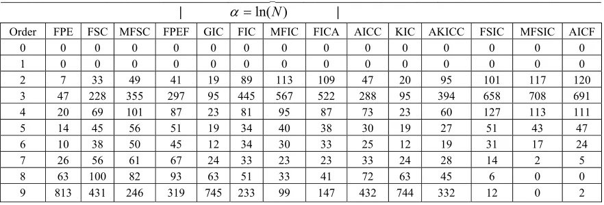
k =(0.9) . The criteria were applied to 1000 independent simulation runs of N=20 samples of the AR(3) process with q_min =0 and q_max =9 as the minimum and maximum candidate orders respectively. The AR estimation method was LSF. The entries of the table show the number of times the order selection criteria chose a particular order out of 1000 trials.

Table 4. Performance comparison of various order selection criteria for an AR(3) process with reflection coefficients k_i =(0.9)i. N is equal to 20, and 0 and 9 are the minimum and maximum candidate

orders respectively. The AR parameter estimation method is LSF. The entries represent the number of times a particular order was selected out of 1000 trials

_____________________________________________________________________________________ | α =ln(N) |

AICF MFSIC FSIC

AKICC KIC

AICC FICA MFIC FIC GIC FPEF MFSC FSC FPE Order

0 0 0 0 0 0 0 0 0 0 0 0 0 0 0

0 0 0 0 0 0 0 0 0 0 0 0 0 0 1

120 117 101 95

20 47 109 113 89 19 41 49 33 7 2

691 708 658 394 95 288 522 567 445 95 297 355 228 47 3

111 113 127 60

23 73 87 95 81 23 87 101 69 20 4

47 43 51 27 19 30 38 40 34 19 51 56 45 14 5

24 17 31 19 12 25 33 30 34 12 45 50 38 10 6

5 2 14 28 24 33 23 23 33 24 67 61 56 26 7

0 0 6 45 63 72 41 33 51 63 93 82 100 63 8

The results presented in tables 1-4 show that the best performance in all cases belongs to MFSIC, closely followed by AICF. However, MFSIC is a semi-empirical criterion and AICF has the best performance among the theoretical criteria (i.e., among the FPE, FPEF, GIC with

α

=

ln(

N

)

, AICC, KIC, AKICC, and AICF criteria). Note that in all cases, the difference between the performance of AICF and the performance of the other theoretical criteria is relatively large. In addition, it can be seen from the tables that the performance of FPEF is always better than that of FPE.

5. CONCLUDING REMARKS

Many of the existing AR model order selection criteria are derived using theoretical or empirical approximations for the expectations of residual variance and prediction error. In this paper, new theoretical approximations were derived for the expectations of residual variance and prediction error. These approximations were used for developing new order selection criteria FPEF and AICF. The FPEF criterion is an estimate of the prediction error and simulation results given in the figures show that, in the finite sample case, it gives much better estimates of the prediction error than FPE. The average value of model error (ME) was used to compare the performance of FPEF and AICF with the existing order selection criteria. In addition, the performance of FPEF and AICF in selecting the correct order was compared with the existing order selection criteria. These comparisons showed that, in the finite sample case, the performance of FPEF is better than that of FPE and, the performance of AICF is much better than those of all existing theoretical order selection criteria. However, MFSIC, which is a semi-empirical criterion, gives a performance that is a little better than that of AICF. In the large sample case, FPEF and AICF become identical with FPE and AIC, respectively. Therefore, FPEF and AICF are (asymptotically) efficient criteria because FPE and AIC are efficient themselves.

REFERENCES

1. Seghouane, A. (2006). Vector autoregressive model-order selection from finite samples using Kullback's symmetric divergence. IEEE Trans. Circuits and Systems, Part I : Regular Papers, 53(10), 2327-35.

2. Hafidi, B. (2006). A small-sample criterion based on Kullback's symmetric divergence for vector autoregressive modeling. Statistics and Probability Letters, 76, 1647-54.

3. Seghouane, A. (2006). A note on overfitting properties of KIC and KICC. Signal Processing, 86, 3055-60. 4. Hafidi, B. & Mkhadri, A. (2006). A corrected Akaike criterion based on Kullback's symmetric divergence:

Applications in time series, multiple and multivariable regression. Computational Statistics and Data Analysis,

50(6), 1524-50.

5. Kay, S. (2005). Exponentially embedded families – New approaches to model order estimation. IEEE Trans. Aerosp. Elect. Syst., 41(1), 333-45.

6. Ridder, F., Pintelon, R., Schoukens, J. & Gillikin, D. P. (2005). Modified AIC and MDL model selection criteria for short data records. IEEE Trans.Instrum. Meas., 54(1), 144-50.

7. Seghouane, A., Bekara, M. & Fleury, G. (2005). A criterion for model selection in the presence of incomplete data based on Kullback's symmetric divergence. Signal Processing, 85, 1405-17.

8. Ing, C. K. & Wei, C. Z. (2005). Order selection for same-realization predictions in autoregressive processes. The Annals of Statistics, 33(5), 2423-74.

9. Stoica, P., Selen, Y. & Li, J. (2004). On information criteria and the generalized likelihood ratio test of model order selection. IEEE Signal Process.Lett., 11(10), 794-97.

11. Shi, P. & Tsai, C. L. (2004). A joint regression variable and autoregressive order selection criterion. Journal of Time Series Analysis, 25(6), 923-41.

12. Akaike, H. (1970). Statistical predictor identification. Ann. Ins. Statist. Math., 22, 203-217.

13. Akaike, H. (1974). A new look at the statistical model identification. IEEE Trans. Autom. Contr., 19(6), 716-723.

14. Hurvich, C. M. & Tsai, C. L. (1989). Regression and time series model selection in small samples. Biometrika,

76, 297-307.

15. Cavanaugh, J. E. (1999). A large-sample model selection criterion based on Kullback's symmetric divergence.

Statist. Probability Lett., 42, 333-343.

16. Seghouane, A. & Bekara, M. (2004). A small sample model selection criterion based on Kullback's symmetric divergence. IEEE Trans. Signal Process., 52(12), 3314-3323.

17. Brockwell, P. J. & Davis, R. A. (1991). Time series: theory and methods.Second ed., New York: Springer-Verlag.

18. Rissanen, J. (1978). Modeling by shortest data description. Automatica, 14, 465-471. 19. Schwarz, G. (1978). Estimating the dimension of a model. Ann. Statist., 6(2), 461-464.

20. Hannan, E. J. & Quinn, B. G.(1979). The determination of the order of an autoregression. J. R. Statist. Soc. Ser. B, B-41, 90-195.

21. Broersen, P. M. T. & Wensink, H. E. (1993). On finite sample theory for autoregressive model order selection.

IEEE Trans. Signal Process, 41(1), 194-204.

22. Broersen, P. M. T. & Wensink,H. E. (1998). Autoregressive model order selection by a finite sample estimator for the Kullback-Leibler discrepancy. IEEE Trans. Signal Process., 46(7), 2058-2061.

23. Karimi,M. (2005). On the residual variance and the prediction error for the LSF estimation method and new modified finite sample criteria for autoregressive model order selection. IEEE Trans. Signal Process., 53(7), 2432-2441.

24. Broersen, P. M. T. (1998). The quality of models for ARMA processes. IEEE Trans. Signal Process., 46(6), 1749-1752.

APPENDIX Using (18), we can write

∑ ∑

∑ ∑

−

= −

= −

= −

= ∧

∧

−

=

+

+

+

+

−

≈

q N

k q N

s

j i s k q

N

k q N

s

g

E

q

N

j

s

q

z

s

q

w

i

k

q

z

k

q

w

E

q

N

j

c

i

c

E

1 1

, , , 2

1 1 2

]

[

)

(

1

)]

,

(

)

(

)

,

(

)

(

[

)

(

1

]

)

(

)

(

[

(A.1)

where g_k,s,i,j is defined as

)

,

(

)

(

)

,

(

)

(

, ,

,

w

q

k

z

q

k

i

w

q

s

z

q

s

j

g

ksij

=

+

+

+

+

(A.2)

In the case where k>s, it is obvious that w(q+k) is independent of w(q+s). In addition, we have shown in section 3 that w(m) is independent of z(n,i) for m≥n. Thus, it is obvious that w(q+k) is independent of

z(q+k,i) and z(q+s,j) for k>s. Therefore, we can write

;

0

)]

,

(

)

(

)

,

(

[

)]

(

[

]

[

g

,,,

E

w

q

k

E

z

q

k

i

w

q

s

z

q

s

j

k

s

E

ksij

=

+

+

+

+

=

>

(A.3)

In the case where s>k, it can be shown in a quite similar way that w(q+s) is independent of the other three variables in the right hand side of (A.2). It follows that

;

0

)]

,

(

)

(

)

,

(

[

)]

(

[

]

[

g

, ,,

E

w

q

s

E

z

q

k

i

w

q

k

z

q

s

j

s

k

In the case that k=s, it follows from (A.2) and (6) that

j

i

k

s

j

k

q

z

i

k

q

z

E

k

q

w

E

j

k

q

z

i

k

q

z

k

q

w

E

g

E

_ksij

≠

=

=

+

+

+

=

+

+

+

=

,

;

0

)]

,

(

)

,

(

[

)]

(

[

)]

,

(

)

,

(

)

(

[

]

[

2 2 ,

, ,

(A.5)

where we have used the fact that w(q+k) is independent of z(q+k,i) and z(q+k,j). It follows from (A.1), (A.3), (A.4), and (A.5) that

; 0 ) ( ) (

[ci c j i j