SELECTION THE BEST CONTROL CHANNEL FOR SSSC STABILIZER TO DAMP INTER-AREA OSCILLATION CONSIDERING NON-LINEARITY EFFECTS

(1)

Printed in The Islamic Republic of Iran, 2012 © Shiraz University

SELECTION THE BEST CONTROL CHANNEL FOR SSSC STABILIZER

TO DAMP INTER-AREA OSCILLATION CONSIDERING

NON-LINEARITY EFFECTS

*

M. R. SHAKARAMI

1

, A. KAZEMI

2

AND M. GITIZADEH

3**

1

Department of Electronics and Electrical Engineering, Lorestan University, Khoramabad, I. R. of Iran

2

Centre of Excellence for Power System Automation and Operation, Department of Electrical Engineering, Iran University of Science and Technology, Narmak, Tehran 16844, I. R. of Iran

3

Department of Electronics and Electrical Engineering, Shiraz University of Technology, Shiraz, I. R. of Iran Email: [email protected]

Abstract– Modal interaction noticeably affects the dynamic behavior of a stressed power system with heavy loading. In this paper, Modal Series (MS) as a method to analyze modal interactions is extended for a power system installed with a static synchronous series compensator (SSSC) stabilizer. The - based and m-based stabilizers as two stabilizers in different control channels are presented for a SSSC. The parameters of the stabilizers are calculated by a quadratic mathematical programming method. In this procedure, the gain and the phase of a stabilizer are calculated simultaneously. A particular measure of stabilizer gain is considered as an objective function. The effects of SSSC based stabilizers on damping inter-area oscillations for a small disturbance are studied and compared. Modal interactions between an inter-area mode and control modes related to SSSC stabilizers are studied by a proposed index based on MS method in a 4-machine stressed power system. Oscillatory instability caused by modal interactions is investigated and compared in the system for both SSSC stabilizers.

Keywords– Inter-area oscillations, static synchronous series compensator (SSSC), damping stabilizer, nonlinear modal interactions, stressed power systems

1. INTRODUCTION

In steady state, SSSC is one of the series flexible AC transmission systems (FACTS) that injects a balanced three phase voltage to a transmission line and quadrature with the line current [1]. Therefore, in this situation it can only exchange the reactive power with the network. Also, in dynamic state it can exchange active power with the network. SSSC when equipped with a suitable stabilizer can damp power oscillations [2]. There are two channels to control the magnitude and phase of the injected voltage. A stabilizer can be applied to both channels to damp mechanical oscillations. For convenience, the stabilizer

in the phase control channel is called - based and in the magnitude control channel is called m-based

stabilizer. In studying small disturbance stability, the - based stabilizer is more effective in damping

inter-area oscillations compared to the m-based stabilizer [3]. When a stressed power system is faced with

partly severe disturbance, nonlinear modal interactions are increased and the dynamic behavior of the system will be complex [4]. In these conditions, modal interactions may deteriorate damping of an inter-area mode and consequently the system may be unstable [5-7]. In past decades, to analyze the modal interactions in stressed power systems, the normal form (NF) method was one of the proposed methods [8-11]. Although the applications of this method are reported in many areas and regarded as a useful and



Received by the editors January 29, 2012; Accepted December 15, 2012. 

(2)

effective tool, there are a few drawbacks to this method. This method needs to do nonlinear transformations as well as solving nonlinear algebraic equations. Also, in this method resonance and quasi-resonance conditions must not be satisfied. Modal series is another method that has been proposed recently to analyze the nonlinear behavior of stressed power systems [12, 13]. The modal series method retains most of the advantages of the NF method, without having the mentioned drawbacks.

Modal interactions in a power system installed with FACTS based stabilizers has not been satisfactorily addressed. Among FACTS devices, the Static VAR Compensator (SVC) and Unified Power Flow Controller (UPFC) have been studied in this field of research [14-18].

In this paper, a lead-lag stabilizer is considered for a SSSC. The gain and phase of the stabilizer are simultaneously calculated by a quadratic mathematical programming method. The modal series method is extended to a power system with a SSSC stabilizer. The approximate responses of a 4-machine power system by linear and modal series methods are compared by a proposed index. Modal interactions between inter-area mode and control modes related to SSSC stabilizers are investigated by a proposed index. Effects of modal interactions on stability of the system with SSSC stabilizer in both control channels are investigated and compared.

2. POWER SYSTEM MODEL

a) Generator

In this study, each generator is represented by a fourth-order d-q axis model. Therefore, nonlinear dynamic

equations for ith generator with known variables are as follows [19]:

s i i





   (1)

) 1 ( )

( )

(         

 

s i qi

i d di qi qi qi di i d mi i

i P I E I E X X I I D

M

 

 (2)

di di di qi FDi qi i

d E E E X X I

T0     (   ) (3)

qi qi qi i d di i

q E E X X I

T₀    (   ) (4)

b) Exciter

In this paper, the IEEE type-AC-4A excitation system is considered, the block diagram is shown in Fig. 1. The role of used parameters for the system is discussed in [20].

R sT 1

1

 B

C sT 1

sT 1

 

A A sT K



1 EFD

T V

REF V

+

-1 E

X

E2

R sT 1

1

 B

C sT 1

sT 1

 

A A sT K



1 EFD

T V

REF V

+

-1 E

X

E2

Fig. 1. Excitation system

c) SSSC modeling

(3)

1 V 2

V L I

2 L

X SCT X_L₁

X Vinj

SC

V m



dc

I V_dc

dc C

1 V 2

V L I

2 L

X SCT X_L₁

X Vinj

SC

V m



dc

I V_dc

dc C

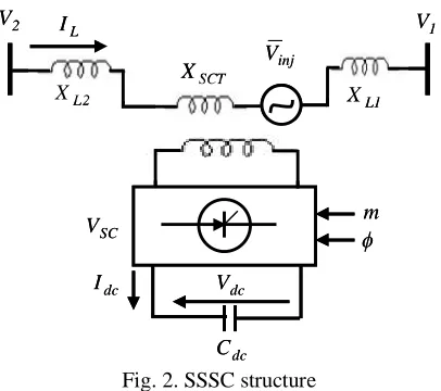
Fig. 2. SSSC structure

The SSSC consists of a series coupling transformer (SCT) with the leakage reactance XSCT, a three-phase

GTO based voltage source converter (VSC) and a DC capacitor. The SSSC can be described as [21]:

j mkV

V_inj  _dc(cos



 sin



) (5)

I jI I

IL  D  Q  L



(6)

I

C

mk

dt

dV

Q D

dc



(

cos





sin



)

₍₇₎

where Vinj is the injected ac voltage by the SSSC; m and  are the modulation ratio and phase defined by

pulse width modulation (PWM), respectively; depending on the converter structure k is the ratio between

the ac and dc voltage; Vdcis the dc voltage; Cdc is the capacitance of the dc capacitor, and ID and IQ are

D-and Q components of the line current IL, respectively.

3. SSSC-BASED STABILIZERS

a) Phase-based stabilizer

Assuming a lossless SSSC, the ac voltage is kept in quadrature with the line current so that the SSSC only exchanges reactive power with the transmission line. By adjusting the magnitude of the injected voltage, the reactive power exchange can be controlled. When the SSSC voltage lags the line current by 90º, it emulates a series capacitor, when the voltage leads the line current by 90º it can also emulate a series inductor. Thus, a SSSC can be considered as a series reactive compensator, where the degree of compensation can be varied by controlling the magnitude of the injected voltage. In this paper, the SSSC is considered in capacitive mode. To keep the injected voltage in quadrature with the line current, a PI

controller, as shown in Fig. 3, has been used. Here, ref is the phase of the injected voltage in steady-state

and its value is considered as ref =-90º+ss , wheress is theangle of the line current in steady-state; Tsssc

is the time constant of the converter, KP and KI are the proportional and integral gains of the PI controller,

respectively. In the PI controller, a lead-lag stabilizer for damping the inter-area oscillations is included. In

this case, the stabilizer is called the phase-based stabilizer and for convenience in this paper, it is called 

-based stabilizer. In this stabilizer, TW is the washout time constant; T is the stabilizer time constant, and x2,

x1 and x0 are parameters to be determined. The feedback signal for the stabilizer is selected among local

(4)

Damping Stabilizer dc V W W sT sT sT x s x s x     1 ) 1 ( 2 0 1 2 2 s K KP  I

SSSC

sT



1

 ref  dcref V + + Vdc max U Vdc min U + + -Input signal Damping Stabilizer dc V W W sT sT sT x s x s x     1 ) 1 ( 2 0 1 2 2 s K KP  I

SSSC

sT



1

 ref  dcref V + + Vdc max U Vdc min U + + -Input signal

Fig. 3.SSSC phase controller with a damping stabilizer

b) Magnitude-based stabilizer

In order to control the magnitude of the injected voltage, the modulation ratio m can be controlled.

Fig. 4 shows the block diagram of the controller in this case, where Xref is the value of produced series

reactance by SSSC in capacitive mode, in steady state condition. A stabilizer for damping of inter-area

oscillations is included in the magnitude controller. This stabilizer is called m-based stabilizer.

ref X SSSC sT  1 1 m × × L

I kV_dc

1 0 1 + Damping Stabilizer W W sT sT sT x s x s x     1 ) 1 ( 2 0 1 2 2 + Input signal ref X SSSC sT  1 1 m × × L

I kV_dc

1 0 1 + Damping Stabilizer W W sT sT sT x s x s x     1 ) 1 ( 2 0 1 2 2 + Input signal

Fig. 4. SSSC magnitude controller with a damping stabilizer

4. QUADRATIC MATHEMATICAL PROGRAMMING TO DESIGN THE STABILIZER

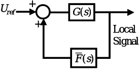
The design method used in this paper is an incremental method including two steps. In the first step, the

closed-loop system is considered as in Fig. 5, where G(s) and F(s) are the power system transfer matrix

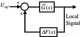
and the stabilizer transfer matrix, respectively. In the second step, the stabilizer transfer matrix is changed

by F. In this case, the closed-loop system changes as shown in Fig. 6, where G(s) is the transfer matrix

of the inner loop between G(s) andF(s).

+ ) (s G ) (s F Local Signal + Uref + ) (s G ) (s F Local Signal + Uref

(5)

+

) (s G

) (s F



Local Signal +

U_ref +

) (s G

) (s F



Local Signal +

U_ref

Fig. 6. Closed loop system in the second step

The details of the method for calculation F are presented in [3]. This method is summarized as

follows. Assuming variations of F are sufficiently small, the variation of the eigenvalue i can be

approximated as:

f

_i

i i





(



)







(i=1, 2, ..., n) (8)

where n is the number of critical eigenvalues and i is the residue associated to the ith eigenvalue i of

) (s

G .

It is assumed that the stabilizer has a lead-lag structure as follows:

w w sT sT sT

x s x s x s f

 

  

1 ) 1 ( )

( 1 ₂ 0

2

2 ₍₉₎

By substituting

s





_i and

x

_m





x

_m(m=1, 2, 3) in (9), the real and imaginary part variations of f (i)

can be obtained as a linear function of x0, x1 and x2. Then, by substituting the real and imaginary parts

of f (i) in (8), the real and imaginary parts of i can be written as a linear function of x0, x1 and x2.

Considering i and i as the desired values of the real and imaginary parts of the critical eigenvalue i,

respectively, the following constraints can be obtained to shift the critical eigenvalues to the desired areas in the complex plane [3].

i i

i



x





x





x







₂ ₂ ₁ ₁ ₀ ₀  (10)

i i

i





x





x





x







   

 ₂ ₂ ₁ ₁ ₀ ₀ (11)

where 0i, 1i, 2i, 0i, 1i, and 2i are specified values. On the other hand, if the angle of residue i is

positive, the stabilizer must have a phase-lead characteristic; otherwise, it must have a phase-lag characteristic. For a phase–lead structure, it is assumed that zeros of the stabilizer are almost one decade closer to the imaginary axis than that of its poles and for the phase-lag structure the zeros are almost one

decade farther to the imaginary axis. Considering

x

_m



x

_m





x

_m(m=1, 2, 3), the constraints on zeros can

be written for a lead-phase stabilizer as in (12) to (14) and for a phase-lag stabilizer as in (15) to (17) [3].

0 2 1 2 0 2 1

2

T

x

T

x

T

x

T

x















(12)

0 2 1

2 0 2 1

2

10

T

x

100

T

x

10

T

x

100

T

x















(13)

0 2 1

2 0

2 1

2

99

180

18

99

180

18



x



T



x



T



x





x



T

x



T

x

(14)

0 2 1 2 0 2 1

2

T

x

T

x

T

x

T

x















(15)

0 2 1 2

0 2 1

2

10

100

10

100

x



T

x



T

x





x



T

x



T

x

(6)

0 2 1

2 0

2 1

2

99

18

180

99

18

180



x



T



x



T



x





x



T

x



T

x

(17)

where

x

0,

x

1and

x

2 are known values.

The following function, as the gain of the stabilizer at the frequency



_i, i=1, 2, . . . m, is considered as the

objective function [3].





2

1

min





m

i

j

f

J



(18)

where



₁,



₂...,



_m are a set of frequencies in the region where the critical eigenvalue must be shifted.

By substituting (9) in (18) and considering

s



j



_i, we can easily rewrite the objective function as

X f X H X 2 1

J __min



T



_ T



₍₁₉₎

where the matrix H and vector f are known and

X

[

x

]

T

0 1 2





is the unknown vector to be

tuned. The objective function (19) along with constraints (10)-(11) and (12)-(14) or (15)-(17) forms a

quadratic mathematical programming problem. To solve this problem, thefunctionof quadprog embedded

inMatab Optimization Toolbox is applied here.

5. ZERO INPUT RESPONSE USING LINEAR AND MODAL SERIES METHODS

The dynamic behavior of a power system can be represented by a set of nonlinear equations as follows:

)

(

X

F

X





(20)

where

X



R

N is the state vector and

F

:

R

N



R

N is a smooth vector field.

Let XSEP be a stable equilibrium point (SEP) of the system. By expanding the Taylor series around XSEP,

the equation (20) can be written as:



 _ _A_X _ _X _H _X _

X T i

i i

2 1

(21)

where Aiis ith row in Jacobeans matrix

SEP

X

F

A

















and

SEP

X l k

i i

x

F

H

















2

is the ith

N



N

sized

hessian matrix.

Let the right and left eigenvectors of matrix A be considered as U and V, respectively. Assuming the

eigenvalues of matrix A are distinct, using the transformation X=UY, equation (21) can be written in the

Jordan form as:



  





 

l k N

k N

l j kl j

j

j y C y y

y

1 1



(22)

where



  

j

kl p

T N

p T jp j

C U H U V

C 





1

2 1

a) Linear modal method

In the linear modal method, only the first term in (21) is considered and higher order terms are

(7)

t jo j j e y t

y ( )  (23)

where yj0 is j

th

element in vector of 1 ₀

0

U

X

Y



 _and_X0_{is the initial condition vector in physical state –}

space.

Using transformation

Y



U

1

X

_{, the approximate solution for}_ith

state variable in the original space would be as: t j N j ij N j j ij i j e y u t y u t

x 0 

1 1 ) ( ) (



  

 (24)

where uij is the i, j element of the right eigenvector matrix U.

b) Modal series method

In this method, beside linear terms, second order terms are also considered, but third and higher order terms are ignored.

In this case, second order closed form approximate solution of (22) for jth state variable in the Jordan form

will be as[12, 13]:

2 2 2 ∈ ) , , ( 1 1 ) , , ( 1 1 ) ( ) , , ( 1 1 0

∑∑

2 2 -) ( R j l k t lo ko N k N l j kl R j l k N k N l t lo ko j kl t R j l k N k N l lo ko j kl j j j l k j te y y C e y y h e y y h y t y                                                                  (25)

where 2 /( k l j)

j kl j kl C

h 











and

R

₂



is all three triples(k,l,j) which satisfy the second order resonance

conditions



k 



l 



j. The second order approximate solution in the physical space can be represented

as:









         N k N l t i kl t N j N j i j i j j ij i l k j _K _e

e t M L t y u t x 1 1 ) ( 1 1 ) ( )

(    ₍₂₆₎

where :





























   



2 ) , , ( 1 1 0 0 0

2

R j l k N k N l l k j kl j i

j

uij

y

h

y

L

2 ) , , ( 1 0

0

∑

2

R j l k N j j kl ij l k i

kl y y u h K             2 ) , , ( 0 0

1 1 _k_l _j _R

l k N k N l j kl ij i

j u C y y

M           



Comparing the coefficients of individual and combination modes in (25) for jth Jordan variable leads to the

(8)

0 0 ,

0

0 0 ,

2 max

2 max )

(

l k j kl l k j

l k j kl l k

y y h y

y y h j

II



 (27)

where ₀ ₀

,

2

max

j _k _l

kl l

k

h

y

is the complex form when

max

,

2

k0 l0

j kl l

k

h

y

occurs.

6. SIMULATION RESULTS

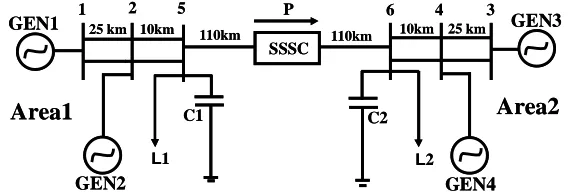
The test system here is a 2-area 4-machine power system. A single line diagram of the system is shown in Fig. 7 [23]. To control inter-area oscillations, a SSSC is installed in the tie-line between nodes 5 and 6. Data of this system and specific parameters used for the SSSC are given in the Appendix. The loads are modeled as constant impedances. No PSS is installed in the system. To increase transferred power, the load in area 2 has been increased and the load in area 1 has then been modified to achieve a given tie-line transferred power.

L1 C1

L2 C2

GEN4 GEN3

GEN2 GEN1

Area1 Area2

SSSC P

1 2 5 6 4 3

25 km 10km _110km _110km 10km 25 km

L1 C1

L2 C2

GEN4 GEN3

GEN2 GEN1

Area1 Area2

SSSC P

1 2 5 6 4 3

25 km 10km _110km _110km 10km 25 km

Fig. 7. One line-diagram of the test system

Table 1. Studied operating conditions

Loading conditions

Load of Area 1(MW)

Load of Area 2(MW)

Transmitted power(MW) Low stress 1000 1300 310

High stress 890 1410 410

Summary of studied operating conditions are shown in Table 1. The oscillation modes in the open loop system for low and high stress loading conditions are shown in Table 2. This table shows that damping of inter-area mode is low, particularly in high stress conditions. To increase damping of this mode to a

desirable value, the parameters of SSSC -based and m-based stabilizers are calculated by a quadratic

mathematical programming method. The variation of line current magnitude is considered as the best input signal for both SSSC stabilizers [3]. As the desired damping ratio for inter-area mode, typically two

values of =7% for high stress loading conditions and =10% for low stress loading conditions have been

considered. The time constant of the stabilizers is considered to be T=0.4 s. Parameters of stabilizers to

achieve desired damping ratios of inter-area mode are shown in Table 3. Loop gains of the stabilizers

(f(j)) in a frequency close to frequency of inter-area mode are shown in the last column of the table.

Typically, this frequency is considered as =1.7 rad/s. This value is average of inter-area mode frequency

for different SSSC stabilizer and different operation conditions. Table 3 shows that for the same desired

damping ratio, the loop gains of the SSSC -based stabilizer is less than the SSSC m-based stabilizer. That

is, to achieve the same desired damping ratio for inter-area mode, control cost in the SSSC -based

stabilizer is lower compared with the SSSC m-based stabilizer. In other words, the SSSC -based

stabilizer is more effective for damping inter-area oscillations. Oscillation modes in closed loop systems

for SSSC and m-based stabilizer are shown in Tables 4 to 6. These tables show that damping ratio of

(9)

Table 2. Oscillation modes in open loop system

Mode #

P=310 MW P=410 MW

Dominant states Eigenvalue Damping (%) Eigenvalue Damping (%)

1,2 -1.225±j7.728 15.66 -1.244±j7.748 15.85 Local, Area 1(1, 2)

3,4 -1.577±j7.451 20.71 -1.554±j7.549 20.16 Local, Area 1(3, 4)

5,6 -0.088±j1.787 4.92 -0.028±j1.647 1.70 Inter-area(1, 2, 3, 4)

7,8 -1.151±j0.846 79.97 -1.320±j0.832 84.60 1,Eq2 ,XE12 ,XE22

9,10 -0.557±j 0.832 55.63 -0.585±j 0.826 57.79 Eq ,Eq4 ,XE14 ,XE24

3

11,12 -0.253±j0.383 55.12 -0.257±j0.393 54.84 Control (Exciter 1) 13, 14 -0.269±j0.358 60.07 -0.284±j0.361 61.79 Control( Exciter 3 and 4)

Table 3. Parameters of SSSC damping stabilizers

P(MW) (%) SSSC stabilize x2 x1 x0 f(j)

410

7 m-based 0.08602 0.04301 0.00538 0.1737 -based 0.00178 0.01169 0.04915 0.0330

10 m-based 0.14440 0.07220 0.00902 0.2915 -based 0.00275 0.03395 0.06764 0.0568

310 10 m-based 0.45702 1.22090 0.47085 1.5337 -based 0.00137 0.00901 0.03837 0.0258

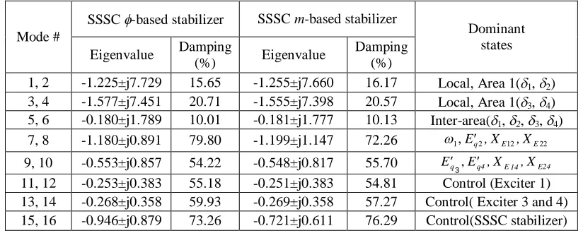
Table 4. Oscillation modes in closed loop system for =10% and P=310 MW

Mode #

SSSC -based stabilizer SSSC m-based stabilizer

Dominant states Eigenvalue Damping

(%) Eigenvalue

Damping (%)

1, 2 -1.225±j7.729 15.65 -1.255±j7.660 16.17 Local, Area 1(1, 2)

3, 4 -1.577±j7.451 20.71 -1.555±j7.398 20.57 Local, Area 1(3, 4)

5, 6 -0.180±j1.789 10.01 -0.181±j1.777 10.13 Inter-area(1, 2, 3, 4)

7, 8 -1.180±j0.891 79.80 -1.199±j1.147 72.26 1,Eq2 ,XE12 ,XE22

9, 10 -0.553±j0.857 54.22 -0.548±j0.817 55.70 Eq₃,Eq4 ,XE14 ,XE24

11, 12 -0.253±j0.383 55.18 -0.251±j0.383 54.81 Control (Exciter 1) 13, 14 -0.268±j0.358 59.93 -0.269±j0.358 57.27 Control( Exciter 3 and 4) 15, 16 -0.946±j0.879 73.26 -0.721±j0.611 76.29 Control(SSSC stabilizer)

Mode #

Dominant states Eigenvalue Damping

(%) Eigenvalue

Damping (%)

1,2 -1.244±j7.749 15.85 -1.250±j7.751 15.91 Local, Area 1(1, 2)

3,4 -1.554±j7.549 20.16 -1.557±j7.548 20.20 Local, Area 1(3, 4)

5,6 -0.123±j1.748 7.02 -0.119±j1.692 7.02 Inter-area(1, 2, 3, 4)

7, 8 -1.402±j0.927 83.42 -1.277±j0.739 86.64 1,Eq2 ,XE12 ,XE22

9, 10 -0.582±j0.854 56.29 -0.584±j0.826 57.73 Eq ,Eq4 ,XE14 ,XE24

3

(10)

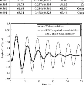
For verification of the designed stabilizers a three-phase fault is applied to the test system at bus 6.

The clearing time of fault, tcr, is set as tcl=20 ms. The fault is cleared without line switching. Because the

generators 1 and 3 have the most contribution in the inter-area mode, typically, swing angle of generator 1 with respect to generator 3 for different SSSC-based stabilizers at high stress operation conditions is shown in Fig. 8. This figure shows that SSSC stabilizers can effectively damp inter-area oscillations.

Mode #

Dominant states Eigenvalue Damping (%) Eigenvalue Damping (%)

1, 2 -1.244±j7.749 15.85 -1.254±j7.751 15.97 Local, Area 1(1, 2)

3, 4 -1.554±j7.549 20.16 -1.559±j7.546 20.24 Local, Area 1(3, 4)

5, 6 -0.172±j1.675 10.21 -0.168±j1.644 10.19 Inter-area(1, 2, 3, 4)

7, 8 -1.453±j0.841 86.54 -1.238±j0.704 86.93 1,Eq2 ,XE12 ,XE22

9, 10 -0.593±j0.862 56.70 -0.584±j0.827 57.68 Eq ,Eq4 ,XE14 ,XE24

3

11, 12 -0.257±j0.393 54.75 -0.257±j0.393 54.82 Control (Exciter 1) 13, 14 -0.283±j0.361 61.68 -0.284±j0.361 61.80 Control( Exciter 3 and 4) 15, 16 -0.568±j0.694 63.34 -0.478±j0.523 67.46 Control(SSSC stabilizer)

0 5 10 15 20 25

1.05 1.1 1.15 1.2 1.25 1.3 1.35 1.4 1.45 1.5

Time (s)

A

n

g

le

(

G

1

-G

3

),

r

ad

Without stabilizer

SSSC magnitude-based stabilizer SSSC phase-based stabilizer

0 5 10 15 20 25

1.05 1.1 1.15 1.2 1.25 1.3 1.35 1.4 1.45 1.5

Time (s)

A

n

g

le

(

G

1

-G

3

),

r

ad

Without stabilizer

SSSC magnitude-based stabilizer SSSC phase-based stabilizer

Fig. 8. Response of system without and with SSSC stabilizer for =10%, P=410 MW and tcl=20 ms

The response of the closed loop system for tcl=15 ms and 40 ms for SSSC -based and m-based

(11)

0 5 10 15 20 25 -0.1

-0.05 0 0.05 0.1 0.15

Time (s)

A

n

g

le

(

G

1

-G

3

),

r

ad

Full solution Modal series approx. Linear approx.

0 5 10 15 20 25

-0.1 -0.05 0 0.05 0.1 0.15

Time (s)

A

n

g

le

(

G

1

-G

3

),

r

ad

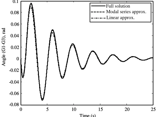
Fig. 9. Response of system with -based stabilizer for =10%, P=410 MW and tcr=15 ms

0 5 10 15 20 25

-0.3 -0.2 -0.1 0 0.1 0.2 0.3 0.4

Time (s)

A

ngl

e

(G

1

-G

3)

,

ra

d

Full solution Modal series approx.

Linear approx.

0 5 10 15 20 25

-0.3 -0.2 -0.1 0 0.1 0.2 0.3 0.4

Time (s)

A

ngl

e

(G

1

-G

3)

,

ra

d

Full solution Modal series approx.

Linear approx.

Fig. 10. Response of system with -based stabilizer for =10%, P=410 MW and tcr=40 ms

0 5 10 15 20 25

-0.08 -0.06 -0.04 -0.02 0 0.02 0.04 0.06 0.08 0.1

Time (s)

A

n

g

le

(

G

1

-G

3

),

r

ad

0 5 10 15 20 25

-0.08 -0.06 -0.04 -0.02 0 0.02 0.04 0.06 0.08 0.1

Time (s)

A

n

g

le

(

G

1

-G

3

),

r

ad

(12)

0 5 10 15 20 25

-0.4 -0.3 -0.2 -0.1 0 0.1 0.2 0.3

Time (s)

A

n

g

le

(

G

1

-G

3

),

r

a

d

0 5 10 15 20 25

-0.4 -0.3 -0.2 -0.1 0 0.1 0.2 0.3

Time (s)

A

n

g

le

(

G

1

-G

3

),

r

a

d

Fig. 12. Response of system with m-based stabilizer for =10%, P=410 Mw and tcr=40 ms

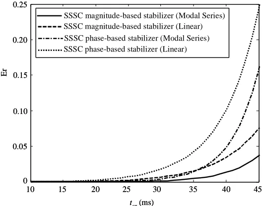
To evaluate the precision of the approximate solutions, an error index is used as follows [24].

dt t x t x T i

Er 



T _i  _i

0 ( )

~ ) ( 1 )

( (28)

where, T is the simulation time, xi(t) and ~x_i(t)are full and approximate response for ith state variable,

respectively.

According to (28), the error index for different values of fault duration for closed loop system in high stress loading conditions for different SSSC stabilizers is shown in Fig. 13. This figure shows that when

fault duration is increased the error index for the system with m-based stabilizer is lower in comparison

with -based stabilizer. In other words, the nonlinear effects are higher in the system with -based

stabilizer. Also, this figure shows that for different values of fault duration, the error index for approximate response obtained by the modal series is lower than the approximate response obtained by the linear method.

10 15 20 25 30 35 40 45

0 0.05 0.10 0.15 0.20 0.25

t_cr(ms)

E

r

SSSC phase-based stabilizer (Modal Series) SSSC phase-based stabilizer (Linear)

SSSC magnitude-based stabilizer (Modal Series) SSSC magnitude-based stabilizer (Linear)

10 15 20 25 30 35 40 45

0 0.05 0.10 0.15 0.20 0.25

t_cr(ms)

E

r

SSSC phase-based stabilizer (Modal Series) SSSC phase-based stabilizer (Linear)

SSSC magnitude-based stabilizer (Modal Series) SSSC magnitude-based stabilizer (Linear)

(13)

According to (27), in some cases, the values of nonlinear modal interaction index for inter-area mode at fault duration of 35 ms are calculated and shown in Tables 7 to 10. According to these tables, the following results can be concluded:

I. According to Table 7, modal interactions between inter-area mode and control modes related

to exciters are not severe in the open loop system.

II. Tables 8 to 10 show that, in the closed loop system, modal interactions between inter-area

mode and control modes related to SSSC stabilizers are higher than that of exciter control modes.

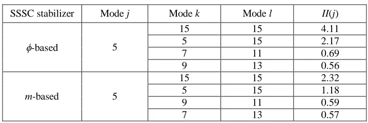
III. Comparing Tables 8 and 10 shows that by increasing stress on the system, modal interactions

between inter-area mode and SSSC stabilizer control modes are increased.

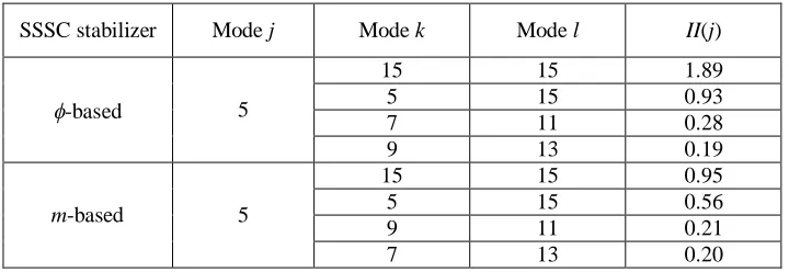
IV. It can be seen from Tables 8 to 10 that modal interactions between inter-area mode and

control mode related to SSSC -based stabilizer are higher than the m-based stabilizer.

V. From Tables 8 and 10, it can be concluded that by increasing desired damping ratio, for

inter-area mode in a certain value of transferred power, the modal interactions between inter-inter-area mode and SSSC stabilizer control modes are increased.

Table7. Nonlinear modal interaction index for inter-area mode in the open loop system for P=410 MW

Mode j Mode k Mode l II(j)

5

5 11 0.62

7 11 0.42

9 13 0.37

5 5 0.11

Table 8. Nonlinear modal interaction index for inter-area mode in the closed loop system for =10% and P=310 MW

SSSC stabilizer Mode j Mode k Mode l II(j)

-based 5

15 15 1.89

5 15 0.93

7 11 0.28

9 13 0.19

m-based 5

15 15 0.95

5 15 0.56

9 11 0.21

7 13 0.20

-based 5

15 15 3.18

5 15 1.72

7 11 0.72

9 13 0.59

m-based 5

15 15 1.84

5 15 0.87

9 11 0.61

(14)

-based 5

15 15 4.11

5 15 2.17

7 11 0.69

9 13 0.56

m-based 5

15 15 2.32

5 15 1.18

9 11 0.59

7 13 0.57

For more stress on the system, loads L1 and L2 are set in the values 1430 and 870 MW, respectively.

In this case, transferred power between two areas is about P=430 MW. The mechanical and control oscillation modes in the open loop system are shown in Table 11. This table shows that inter-area mode is unstable for this condition. Mechanical and control modes in the closed loop system, with parameters of

Table 3 related to P=410 MW and =10%, are presented in Table 12. This table shows that damping ratio

of inter-area mode in the closed loop system has been reduced by increasing transmitted power. Also, it

can be seen from this table that the damping of inter-area mode with the -based stabilizer is somewhat

higher than the m-base stabilizer. Swing angle of generator 1 with respect to generator 3 for the -based

and m-based stabilizer at different values of fault duration are shown in Figs. 14 and 15, respectively.

Figure 14 shows that when fault clearing time is 10 ms (small disturbance) the system is stable. This

condition is coincident with eigenvalue results. By increasing fault duration to tcr=25.3 ms, damping of

oscillations would be approximately zero and the oscillations are repeated periodically without decaying or diverging. Lastly, in fault duration of 26.5 ms, the system is faced with oscillatory instability and loses its synchronism after about 20 seconds.

Table 11. Oscillation modes in the open loop system for P=430 MW

Mode # Eigenvalue Damping (%) Dominant states 1,2 -1.247±j7.760 15.87 Local, Area 1(1, 2)

3,4 -1.539±j7.585 19.88 Local, Area 1(3, 4)

5,6 0.024±j1.476 -1.63 Inter-area(1, 2, 3, 4)

7, 8 -1.431±j0.718 89.38 1,3,Eq2 ,XE12 ,XE22

9, 10 -0.584±j0.822 57.92 Eq ,Eq4 ,XE14 ,XE24

3

11, 12 -0.257±j0.397 54.34 Control (Exciter 1) 13,14 -0.288±j0.361 62.36 Control( Exciter 3 and 4)

Table 12. Oscillation modes in the closed loop system (with parameters of Table 3 related to P=410 MW and =10%) for P=430 MW

Mode # SSSC -based stabilizer SSSC m-based stabilizer Dominant states

Eigenvalue Damping (%) Eigenvalue Damping (%)

1,2 -1.246±j7.760 15.85 -1.256±j7.763 15.97 Local, Area 1(1, 2)

3,4 -1.539±j7.585 19.88 -1.543±j7.583 19.94 Local, Area 1(3, 4)

5,6 -0.052±j1.432 3.63 -0.043±j1.419 3.03 Inter-area(1, 2, 3, 4)

7, 8 -1.662±j0.684 92.47 -1.224±j0.616 89.33 1,3,Eq2 ,XE12 ,XE22

9, 10 -0.595±j0.859 56.94 -0.580±j0.823 57.61 Eq₃,Eq4 ,XE14 ,XE24

(15)

0 5 10 15 20 25 -0.4 -0.3 -0.2 -0.1 0 0.1 0.2 0.3 0.4 0.5 0.6 Time (s) A n g le ( G 1 -G 3 ), r ad

tcl=10 ms

tcl=25.3 ms

tcl=26.5 ms

0 5 10 15 20 25

-0.4 -0.3 -0.2 -0.1 0 0.1 0.2 0.3 0.4 0.5 0.6 Time (s) A n g le ( G 1 -G 3 ), r ad

tcl=10 ms

tcl=25.3 ms

tcl=26.5 ms

Fig. 14. Response of the system for SSSC -based stabilizer (with parameters of Table 3 related to P=410 MW and =10%) for P=430 MW at different values of fault duration

0 5 10 15 20 25

tcl=10 ms

tcl=26.5 ms

t_cl=32.3 ms

0 5 10 15 20 25

tcl=10 ms

tcl=26.5 ms

t_cl=32.3 ms

Fig. 15. Response of the system for SSSC m-based stabilizer (with parameters of Table 3 related to P=410 MW and =10%) for P=430 MW at different values of fault duration

The fault clearing time for first swing instability for both SSSC stabilizers is shown in Fig. 16. Comparing Figs.14 and 16, it can be seen that fault clearing time for oscillatory instability is about 8 ms less than the

clearing time for the first swing instability. Figure 15 shows that the system with SSSC m-based stabilizer

at tcl=26.5 ms is stable (unlike -base stabilizer). Also, comparing this figure to Fig. 16 shows that fault

clearing time for instability of the system is close to that of for first swing instability.

0 5 10 15 20 25

-0.5 0 0.5 1 1.5 2 2.5 3 Time (s) A n gl e (G 1 -G 3), ra d

SSSC magnitude-based stabilizer with tcr=35.18 ms

SSSC phase-based stabilizer with tcr=34.48 ms

0 5 10 15 20 25

-0.5 0 0.5 1 1.5 2 2.5 3 Time (s) A n gl e (G 1 -G 3), ra d

SSSC magnitude-based stabilizer with tcr=35.18 ms

SSSC phase-based stabilizer with tcr=34.48 ms

(16)

ForP=410 MW, modal interaction index between inter-area mode and SSSC stabilizer control modes for

fault duration of 25 ms is shown in Table 13. This table confirms that modal interactions for SSSC 

-based stabilizer are severe in comparison with m-based stabilizer.

It can be seen from the above results that modal interactions can deteriorate damping of a mechanical mode that causes the system to become unstable. However, the system is recognized as stable due to a small disturbance.

Table 13. Nonlinear modal interaction index for inter-area mode in the closed loop system (with parameters of Table 3 related to P=410 MW and =10%) for P=430 MW

SSSC

stabilizer Mode j Mode k Mode l II(j)

-based 5

15 15 5.68

5 15 3.17

7 11 0.98

9 13 0.86

m-based 5

15 15 3.38

5 15 2.10

9 11 1.06

7 13 0.92

7. CONCLUSION

In this paper, modal series method is extended to a multi-machine power system installed with a SSSC-based stabilizer. Phase and magnitude control channels are considered for the SSSC stabilizer. Parameters of the SSSC stabilizer are calculated by a quadratic mathematical programming method. Results show that for small disturbance analysis (eigenvalue analysis), the gain (the control cost) of the stabilizer to improve

damping of an inter-area oscillation mode to a desired value with SSSC -based stabilizer is less than the

m-based stabilizer. By increasing the fault duration (magnitude of disturbance) in certain operating

conditions, modal interactions between inter-area mode and control mode related to SSSC -based

stabilizer are higher than the m-based stabilizer. Also, results show that in a certain heavy loading

condition, the system with -based stabilizer is faced with an oscillatory instability whose clearing time is

less noticeable than that for the first swing instability. Therefore, to select the optimal control channel for a SSSC stabilizer, in stressed power systems in which modal interactions between an inter-area mode and control modes are high, eigenvalue analysis (small disturbance analysis) alone may not be sufficient and effects of modal interactions must be considered. In other words, a trade-off between linear and nonlinear analysis must be done.

REFERENCES

1. Gyugyi, L., Schauder, C. D. & Sen, K. K. (1997). Static synchronous series compensator: a solid-state approach to the series compensation of transmission lines. IEEE Trans. Power. Deliv., Vol. 12, No. 1, pp. 406-417. 2. Ghaisari, J. & Bakhshai, A. (2006). An advanced robust MIMO SSSC control technique for power oscillation

damping improvement. Iranian Journal of Science and Technology, Transaction B: Engineering, Vol. 30, No. B6, pp. 667-679.

3. Shakarami, M. R. & Kazemi, A. (2011). Assessment of effect of SSSC stabilizer in different control channels on damping inter-area oscillations, energy. conver. manag., J., Vol. 52, No. 3, pp. 1622-1629.

4. Vittal, V., Bhatia, N. & Fouad, A. A. (1991). Analysis of the inter-area mode phenomenon in power systems following large disturbances. IEEE Trans. Power Syst., Vol. 6, No. 4, pp.1515-1521.

(17)

6. Amano, H., Kumano, T. & Inoue, T. (2006). Nonlinear stability indexes of power swing oscillation using normal form analysis. IEEE Trans. Power Syst., Vol. 21, No. 2, pp. 825-834.

7. Amano, H. & Inoue, T. (2007). A new PSS parameter design using nonlinear stability analysis. IEEE, Power Engineering Society General Meeting, Tampa, Florida.

8. Lin, C. M., Vittal, V., Kliemann, W. & Foad, A. A. (1996). Investigation of modal interaction and its effects on control performance in stressed power systems using normal forms of vector fields. IEEE Trans. Power Syst., Vol. 11, No. 2, pp. 781-787.

9. Jang, G., Vittal, V. & Klimann, W. (1998). Effect of nonlinear modal interaction on control performance: Use of normal forms technique in control design, Part I: General theory and procedure. IEEE Trans. Power Syst., Vol. 13, No. 2, pp. 401-407.

10. Jang, G., Vittal, V. & Klimann, W. (1998). Effect of nonlinear modal interaction on control performance: Use of normal forms technique in control design, Part II: Case studies. IEEE Trans. Power Syst., Vol. 13, No. 2, pp. 408-413.

11. Thapar, J., Vittal, V., Kliemann, W. & Foad, A. A. (1998). Application of the normal form of vector fields to predict inter-area separation in power systems. IEEE Trans. Power Syst., Vol. 2, No. 2, pp. 844-850.

12. Shanechi, H. M., Pariz, N. & Vaahedi, E. (2003). General nonlinear modal representation of large scale power systems. IEEE Trans. Power Syst., Vol. 18, No. 3, pp.1103-1109.

13. Pariz, N., Shanechi, H. M. & Vaahedi, E. (2003). Explaining and validating stressed power systems behavior using modal series. IEEE Trans. Power Syst., Vol. 18, No. 3, pp. 778-785.

14. Zou, Z. Y., Jiang, Q. Y., Cao, Y. J. & Wang, H. F. (2005). Application of the Normal Forms to analyze the interactions among the multiple-control channel of UPFC. Int. J. Electric Power Energy Syst., Vol. 27, No. 8, pp. 584-593.

15. Soltani, S., Pariz, N. & Gazi, R. (2009). Extending the perturbation technique to the modal representation of nonlinear systems. Elect. Pow. Syst. Res., Vol. 79, No. 8, pp. 1209-1215.

16. Messina, A. R. & Barocio, E. (2003). Nonlinear analysis of inter-area oscillations: Effect of SVC voltage support. Elect. Pow. Syst. Res., Vol. 64, No. 1, pp. 17-26.

17. Barocio, E. & Messina, A. R. (2003). Normal form analysis of stressed power systems: incorporation of SVC models. Int. J. Elect. Pow. Energy Syst., Vol. 25, No. 1, pp. 79-90.

18. Zou, Z. Y., Jiang, Q. Y., Cao, Y. J. & Wang, H. F. (2005). Normal form analysis of interactions among multiple SVC controllers in power systems. IEE Proc. Gener. Transm. Distrib., Vol. 152, No. 4, pp. 469-474.

19. Sauer, P. & Pai, M. (1998). Power system dynamics and stability. Prentice Hall, New Jersey.

20. Anderson, P. M. & Fouad, A. A. (1977). Power system Control and stability. Iowa, Iowa State Univ.

21. Wang, H. F. (2000). Static synchronous series compensator to damp power system oscillation. Elect. Pow. Syst. Res., Vol. 54, No. 2, pp. 113-119.

22. Naghshbandy, A. (2008). Study of fault location effects on low frequency inter-area oscillations in stressed power systems. Dissertation, Iran University of science and technology, Iran.

23. Liu, S., Messina, A. R. & Vittal, V. (2005). Assessing placement of controllers and nonlinear behavior using normal form analysis. IEEE Trans. Power Syst., Vol. 20, No. 3, pp. 1486-1495.

24. Wu, F. X., Wu, H., Han, Z. X. & Gan, D. Q. (2007). Validation of Power system non-linear modal analysis methods. Elect. Pow. Syst. Res., Vol. 77, No. 10, pp. 1418-1424.

APPENDIX A: Data used for simulations

Data of SSSC (in p.u. except indicated): TSSSC=0.01 s, k=1, XSCT=0.15, CDC=1, Vdcref=1, Xref=0.12, KP=25, KI=200. Data of generator and network:

1. Synchronous generator data: Table A1.

(18)

3. Exciter parameters: Table A2.

4. Load flow data (in p.u.) on base 100 MVA): QC1=2.551, QC2=2.543, Ql1=2.50,Ql2=2.50, Pg1=6.644,

Pg2=6.644, Pg4=5, V3=1.020 (swing bus), |V1|=1.02, |V2|=1.02, |V4|=1.02.

Table A1. Generator data (in p.u. except indicated)

Parameter G1 G2 G3 G4

Ra 0.0025 0.0025 0.0025 0.0025

xd 1.8 1.8 1.8 1.8

xq 1.7 1.7 1.7 1.7