Printed in The Islamic Republic of Iran, 2008 © Shiraz University
GLOBAL PASSIVITY ENFORCEMEN
TVIA CONVEX OPTIMIZATION
*B. PORKAR
1, M. VAKILIAN
1* *AND S. M. SHAHRTASH
21Dept. of Electrical Eng., Sharif University of Technology, Tehran, I. R. of Iran
Email: [email protected]
2 Dept. of Electrical Eng., Iran University of Science and Technology, Tehran, I. R. of Iran
Abstract– Application of the network equivalent concept for external system representation for power system transient analysis is well known. However, the challenge to utilize an equivalent network, approximated by a rational function, is to guarantee the passivity of the corresponding model. In this regard, special techniques are required to enforce the passivity of the equivalent model through a post processing approach that minimizes its impact on the original model characteristics. In this paper, the passivity is enforced by expressing the problem in terms of a convex optimization problem that guarantees the global optimal solution. The convex optimization problem is efficiently solved by recently developed numerical interior–point methods. This passivity enforcement is also global which indicates that the passivity enforcement in one region does not lead to passivity violation in other regions.
Keywords– Optimization, globally optimal (minimum perturbation) solutions, global passivity enforcement, network equivalents, power system components
1. INTRODUCTION
Applications of network equivalents for the representation of external systems in production grade time domain electromagnetic transients programs result in significant reduction in CPU memory and run time. A number of methods have been proposed for the construction of a network equivalent. These methods can be categorized into time domain equivalent and frequency domain equivalent methods. The solution in the frequency domain is essentially aimed to identify rational functions that approximate the admittance matrix of the external system seen from the boundary node(s). Among various fitting methods, the Vector Fitting (VF) has proved its efficiency and accuracy for different applications [1-6]. It permits identification of state space models directly from the measured or computed frequency responses for both single and multiple input/output systems. Although VF can lead to a stable and precise approximation, the corresponding model may not be passive. A stable, but non-passive network in association with passive networks or loads may lead to an unstable system. Therefore passivity is a required property for a model, although its enforcement is a difficult task.
In [7-9] the passivity violation regions are detected via a purely algebraic method, based on the existence of purely imaginary eigenvalues of associated Hamiltonian matrices obtained from the state-space representation of a reduced-order model. This method overcomes drawbacks of the frequency sweep method first presented in [10], for computation of the H∞ norm of a transfer matrix. The perturbation or compensation stage to enforce passivity in [7] aims at displacement of the imaginary eigenvalues of the Hamiltonian matrix, based on the first-order perturbation theory and via an iterative perturbation scheme. However, only when the passivity violations are of small-signal nature is the method efficient, having the
least impact on the system behavior. Furthermore, it does not provide any guarantee of a globally optimal (minimum perturbation) solution. In [8], the passivity correction (compensation) is performed at the frequency point of maximum violation in a non-passive region by slightly perturbing the residue matrix based on the first-order perturbation theory. It is also shown in [8] that if only the diagonal elements of the residue matrix are considered for perturbations, the passivity enforcement is global, i.e. passivity enforcement in one region does not lead to passivity violation in other regions.
Passivity is also enforced by introducing the passivity criterion as a constraint equation of a least squares problem to be solved based on a Quadratic Programming (QP) approach, using Newton’s method [11]. The constraint equation is formed based on nonnegative definiteness of the Hermitian part of the transfer function, at the frequency points of the passivity violation regions, as detected via frequency sweep. However this method cannot guarantee global passivity. To overcome this drawback, the process is performed in an iterative manner, although it does not reliably ensure passivity.
In this paper, the passivity enforcement problem is formulated as a convex optimization problem and efficiently solved based on recently developed interior-point methods. The convex optimization is a special class of mathematical optimization problems in which the objective and constraint functions are all convex. While the theoretical properties of convex optimization problems have been well established, their merits for practical applications are only beginning to emerge. The main reason is the recent developments of powerful interior-point methods for general convex optimization problems. These methods can efficiently solve large size problems, with thousands of variables and tens of thousands of constraints, within a reasonable time, using a conventional CPU. Moreover, the solution found by these methods is guaranteed to be the global solution, irrespective of the initial point (which, indeed, need not be feasible). This is in contrast to the locally optimal solutions produced by most numerical optimization methods.
2. PROBLEM FORMULATION
a) Input-output transfer function matrix
A linear time-invariant (LTI) multi-port system can be converted into the conventional state-space form as:
( )
( )
( )
( )
t Cx( )
t Du( )
t yt Bu t Ax t x
+ =
+ =
&
(1)
where, x(t)∈ℜn: the state vector, u,y∈ℜp: input and output vectors,A∈ℜn×n,B∈ℜn×p, C∈ℜp×n and . The number of ports and the dynamic order of the approximated function are p and n , respectively. Poles and residues of the system are determined by matrices A and C, respectively. The input-output transfer function matrix of the system can be obtained from (1) as:
p p
D∈ℜ ×
Y
( ) (
s =C sI −A)
−1B+D (2) where s is the Laplace operator.b) Rational approximation via vector fitting (VF)
In the frequency domain, the linear time-invariant (LTI) system of (2) can be represented by a rational pole-residue model as
( )
∑
=
+
+
−
=
Nm m
m
D
sE
a
s
R
s
Y
1
This model can be obtained by various approaches, e.g. via Vector Fitting (VF). Conceptually, VF is a pole relocation technique where the poles are improved based on an iterative process. This is achieved by repeatedly solving a sequence of linear problem until convergence is achieved. The VF formulation avoids ill-conditioning problems, and the formulation is given by simple fractions (instead of polynomials). In [12], this approach is recognized as a reformulation of the Sanathanan-Koerner (SK) iteration [13]. The orthonormal vector fitting technique, introduced in [14], improves numerical stability of VF by using orthonormal rational functions. This leads to better conditioned equations that significantly reduce numerical sensitivity to the choice of starting poles, and reduces the number of iterations, which in turn reduces the overall computation time.
c) Definition of passivity
Passivity may be loosely defined as the inability of a given system to generate energy. The precise definition of passivity requires that the transfer matrix representing the system admittance be positive real. This condition requires that the Hermitian part of the transfer matrix be nonnegative definite on the imaginary axis, i.e.,
( )
ω =(
( )
ω + ∗( )
ω)
≥0 ∀ω2 1
j Y j Y j
G (4)
where denotes complex conjugate transpose. Condition (4) can be verified by ensuring that all its eigenvalues are nonnegative at any frequency:
∗
( )
ω λ( )
ω λ(
( )
ω)
ωλi j ≥0 ∀ i j ∈ G j ∧∀ (5)
The direct application of the definition (5) for testing passivity, however, requires a frequency sweep since this condition needs to be checked at all frequencies. The results of such a test, therefore, depend on the accurate sampling of the frequency axis, which is not a trivial task. For this reason, purely algebraic passivity tests are highly desirable and will be described in section V.
3. CONVEX OPTIMIZATION
a) Optimization methods
The goal of this section is to highlight the potential merits of the position of convex optimization methods with respect to other optimization methods.
1) The main general-purpose classical optimization methods include Steepest Descent, Quadratic Programming (QP), Sequential Quadratic Programming (SQP), Lagrange Multiplier (Kuhn-Tucker Conditions), and Gradient Projection methods (Generalized Reduced Gradient (GRG) methods). The main feature associated with these methods is their capability to handle a wide variety of problems; the only requirement is that the performance measures, along with one or more derivatives, should be computed. The main limitation of the classical optimization methods is that they converge to locally optimal solutions.
do not require the calculation of derivatives. The main drawback of a knowledge-based method is that it provides a local, not global, optimal solution.
3) The most widely known global optimization methods are branch and bound and Simulated Annealing (SA). The main drawback of these methods is that they need significant CPU time for a realistic size problem, as is the case for power system optimization problems.
A convex optimization problem is a special optimization problem in which the objective and constraint functions are all convex. In this respect, the salient feature of interior-point methods is their (i) significant efficiency to solve convex optimization problems, and (ii) capability to obtain the global optimum, irrespective of the starting point of the optimization process. The initial point does not need to be a feasible point.
b) Convexity and its properties
A set C is convex if the line segment between any two points in C lies in C, i.e. for any and any
C
x
x
1,
2∈
θ
with0
≤
θ
≤
1
we haveθ
x
1+
(
1
−
θ
)
x
2∈
C
. A function f is convex on a convex set if(
)
(
x
y
)
f
( ) (
x
) ( )
f
y
f
θ
+
1
−
θ
≤
θ
+
1
−
θ
.A convex optimization problem (or a convex program) is the minimization of a convex function over a convex set. It can be shown that any local minimum of a convex function is a global minimum. The affine functionsaTx+b, where a, x are vectors and b is a scalar; quadratic functions xTRx (provided that
R is a symmetric positive semi-definite matrix), and norms of vectors ||x|| (which include the Euclidean norm, the absolute value, and the maximum value of a set of elements), are samples of convex functions.
An upper bound on a convex function yields a convex set, i.e. if function f is convex and , then is convex. A lower bound on a convex function is not a convex constraint in general.
R a∈ }
) ( |
{x f x ≤a
c) Interior point methods
Originally IPMs were proposed by von Neumann [16], Hoffman et al. [17] and Frisch [18] based on the logarithmic barrier method at almost the same time Dantzig presented the famous simplex method. However the main initiation in the application of IPMs is recorded under the name of Karmarkar [19], who came up with a novel IPM based on nonlinear projective transformations that were able to solve large-scale linear programs (LP) up to 50 times faster than the simplex method. IPMs are usually classified into: i) projective methods [19-21] based on Karmarkar's original algorithm, ii) affine-scaling methods [22] obtained as simplifications of projective methods, and iii) primal-dual methods [23, 24] that have emerged as the most useful methods. The major primal-dual methods are considered as path-following methods [23], potential-reduction methods [25], and infeasible-interior-point methods [26].
Among the different IPMs appearing in the literature [27], the infeasible-primal-dual log barrier methods are considered and referred to as the most effective ones for solving large-scale problems [24]. The name infeasible-interior-point primal-dual is due to the algorithm generating iterations which are interior, with respect to the inequality constraints, but do not necessarily satisfy the equality constraints.
A general framework for solving nonlinear convex optimization problems using interior point methods has been described in [23] and [28, 29]. The work presented in [28] extends the theory of linear programming interior-point methods to nonlinear convex optimization problems using the convergence theory of Newton's method for self-concordant functions. In this section we briefly explain interior-point methods for solving convex optimization problems that include inequality constraints as follows:
minimize
f
0( )
x
where f0,…, fm :
R
n→
R
are convex and twice continuously differentiable, andA
∈
R
p×nwith a rank of A= p < n. Interior-point methods solve problem (6) by applying Newton’s method to a sequence of equality constrained problems. We consider a particular interior-point algorithm which is called the barrier method. The first step is to rewrite (6), making the inequality constraints implicit in the objective function, as follows:
minimize
( )
+
∑
m= −(
( )
)
i
I
f
ix
x
f
1
0 (7) subject to Ax = b
where
I
−:
R
→
R
is the indicator function for real, non-positive
( )
⎩ ⎨ ⎧
> ∞
≤ =
− 0
0 0
u u u
I
The basic idea of the barrier method is to approximate the indicator function
I
− by a function, e.g.( ) ( ) ( )
− ++ − u =− t −u dom I =−RIˆ 1 log , ˆ (8)
where is a parameter that sets the accuracy criterion for the approximation. Similar to , is also a convex and non-decreasing function, and (according to the convention) takes on the value of
0
>
t
I
− Iˆ−∞ for . Unlike , however, is differentiable and closed, i.e. it increases to ∞ as
u
approaches 0. Substituting for in (7) results in:0
>
u
I
− Iˆ−−
Iˆ
I
−minimize
f
0( )
x
+
∑
im=1−
( )
1
t
log
(
−
f
i( )
x
)
subject to Ax = b, (9)
Function
( )
x
=
−
∑
mi=1log
(
−
f
i( )
x
)
φ
(10)with
dom
{
x
R
nf
i( )
x
0
,
i
1
,
,
m
}
K
=
<
∈
=
φ
, called the logarithmic barrier or log barrier for (9). If parameter t is large, it is difficult to minimize functionf
0+
( )
1
t
φ
using Newton’s method. The reason is that its Hessian varies rapidly in the vicinity of the boundary of the feasible set. This can be circumvented by solving a sequence of problems, formulated in the same form as (9), by increasing parameter t (and therefore the accuracy of the approximation) at each step, and starting each new minimization process from the solution corresponding to that value of t obtained from the previous solution. If the objective function is multiplied by t, the equivalent problem can be considered as:minimize
tf
0( ) ( )
x
+
φ
x
subject to Ax = b (11)
which provides the same results. For
t
>
0
,x
∗( )
t
can be defined as the solution of (11). The central path associated with (11) is defined as a set of pointsx
∗( )
t
, , which are called the central points. Pointson the central path are characterized by the following necessary and sufficient conditions: is strictly feasible, i.e. satisfies
0
>
t
( )
t
x
∗( )
t
b
f
( )
x
( )
t
i
m
Ax
∗=
,
∗<
0
,
=
1
,
K
,
( )
( )
( )
( )
( )
( )
( )
( )
( )
( )
ν
ν
φ
ˆ 1 ˆ 0 1 0 0 T i m i i T A t x f t x f t x f t A t x t x f t + ∇ − + ∇ = + ∇ + ∇ = ∗ = ∗ ∗ ∗ ∗∑
(12)From (12), an important property of the central path can be derived as follows: Every central point yields a dual feasible point, and hence a lower bound exists on the optimal value of
p
∗as:
( )
( )
( )
x t i m( )
t ttf t i i
ν
ν
λ
=− 1 , =1, , , ∗ = ˆ∗ ∗
K (13)
It can be shown that the pair
λ
∗i( ) ( )
t ,ν
∗ t is a dual feasible pair. Hence dual function g(
λ
∗i( ) ( )
t ,ν
∗ t)
is finite, and
(
( ) ( )
)
( )
( )
( )
( )
( )
( )
(
( )
)
( )
( )
x
t
m
t
f
b
t
Ax
t
t
x
f
t
t
x
f
t
t
g
m i T i i i−
=
−
+
+
=
∗ = ∗ ∗ ∗ ∗ ∗ ∗ ∗∑
0 1 0,
ν
λ
ν
λ
(14)
This indicates that the duality gap is associated with
x
∗( )
t
and the dual feasible pairx
∗( )
t
,ν
∗( )
t
is simply m/t. Therefore, we have(
x( )
t)
p m t (15)f ∗ − ∗ ≤
0
i.e.,
x
∗( )
t
is not larger than m/t-(sub-optimal solution). This confirms the intuitive idea that x∗( )
tconverges to an optimal point as . This also suggests a very straightforward method for solving (11) with a guaranteed pre-specified accuracy
∞
→
t
ε
. By assumingt
=
m
ε
, the equality constrained problem can be solved by a Newton’s method, asminimize
(
m
ε
) ( ) ( )
f
0x
+
φ
x
subject to Ax = b (16)
where
x
∗( )
t
is computed for a sequence of increasing values of t, untilt
≥
m
ε
, which guarantees thatε
-suboptimal solution of the original problem is achieved. The proposed algorithm for application to the method is as follows:Given: strictly feasible
x
,
t
:
=
t
(0)>
0
,
μ
>
1
,
toleranceε
>
0
Repeat:
1. Setting the central path.
Compute
x
∗( )
t
by minimizing+
φ
0tf
, subject to Ax = b, and starting at x. 2. Update.x
:
=
x
∗( )
t
.3. Stopping criterion. quit if
m
t
<
ε
. 4. Increase t as follows:t=µt, (µ>1).
The highlights related to the choice of
μ
and have been discussed in [30]. Primal-dual interior-point methods are often more efficient than the barrier method, especially when high accuracy is required, since they can exhibit a better convergence rate than linear type methods [24, 31].) 0 (
t
15 thousand C source lines of code, is a highly sophisticated and public-domain solver. It has been developed by C. Meszaros [33] and recently implemented in MATPOWER [34] via a MATLAB MEX interface. BPMPD is based on Methrotra's predictor-corrector [35] and has been equipped with warm-start producer and sparse techniques. The values for
μ
and are internally selected by the solver. In this paper, the passivity enforcement problem is first formulated as a Quadratic Programming (QP) problem, and then it is solved by an efficient implementation of infeasible-interior-point primal-dual method, through the BPMPD solver.) 0 (
t
4. PASSIVITY ENFORCEMENT PROBLEM
In this section, the passivity enforcement problem is formulated as a convex optimization problem and solved by using interior-point methods. As described in section II.C, the passivity criterion implies that eigenvalues of the real part of the admittance matrix Yare positive for all frequencies:
(Re{
})
0
1
>
+
+
−
∑
=
N
m m
m
D
sE
a
s
R
eig
(17)This criterion can be enforced by perturbing the model parameters that minimizes its impact on the original model, i.e. [11]
0
1
≅
Δ
+
−
Δ
=
Δ
∑
=
N
m m m
D
a
s
R
Y
(18)
(Re{
})
0
1
>
Δ
+
−
Δ
+
∑
=
N
m m m
D
a
s
R
Y
eig
(19)This leads to the following convex optimization problems in a quadratic form of [11]
minimize
Δ
x
TA
sysTA
sysΔ
x
subject to BsysΔx<c (20)
or in a linear form of
minimize AsysΔx
subject to BsysΔx<c (21)
where vector c includes magnitudes of eigenvalues of the real part of Y at all frequency points, and Asys
includes coefficients of residues (elements of R) and constant terms (elements of D) at all frequency points. BBsys [11] can be computed only at frequency points where passivity violations are detected via a
frequency sweep. This method cannot guarantee global passivity since BsysB is to be evaluated at all
frequency points within the approximation range. However, passivity violations may appear outside the fitting range. This drawback can be overcome by accurate detection of passivity violation regions via the pure algebraic method described in section V. If the region(s) of passivity violation is(are) outside the fitting range, the inequality constraint can also be extended to those frequency points. Thus, the global passivity is ensured. This approach may result in a large size problem, however, it can be efficiently solved by interior-point methods. Therefore the following algorithm is proposed to enforce the global passivity.
• Detect the passivity violation regions (section V). • Set up the convex optimization problem.
)
• Check the passivity violation (section V). If these still are passivity violation regions, repeat the process.
5. CHARACTERIZATION OF PASSIVITY VIOLATIONS
With respect to the proposed algorithm of the previous section, we need to precisely identify the passivity violation regions. Hence, in this section we introduce a purely algebraic method based on Hamiltonian matrices associated with the state-space realization. This technique was first presented in [10] and then used in [8, 9]. Let us first recall the definitions of the Hamiltonian matrices for hybrid cases (with emphasis on Y form for network equivalent applications)
(22) where
(
)
(
) (
⎟⎟ ⎠ ⎞ ⎜⎜ ⎝ ⎛ − − − + = + − ⎟⎟ ⎠ ⎞ ⎜⎜ ⎝ ⎛ − + ⎟⎟ ⎠ ⎞ ⎜⎜ ⎝ ⎛ − = − − − − − T T T T T T T T T B Q C A C Q C B BQ C BQ A B C D D I C B A A N 1 1 1 1 1 2 0 0δ
δ(
I
D
D
T)
Q
=
2
δ
−
−
.δ
N
is a Hamiltonian matrix, indicating thatJ N J NT where
δ δ =− −1
⎟⎟
⎠
⎞
⎜⎜
⎝
⎛
−
=
0
0
I
I
J
and denotes transpose. T
N
δ depends on scalar parameter δ which is related to the spectrum offrequency-dependent eigenvalues of Y and expressed by the following theorem.
Theorem: Assume A has no imaginary eigenvalues,δ is not a singular value of
(
D
+
D
T)
2
and∈
R
0
ω
.Then, δ is an eigenvalue of
G
( )
j
ω
if and only if(
N
δ−
j
ω
0I
)
is singular[10]. A passivity test can be readily designed by using the critical level δ =0 and hence
(
)
(
)
(
)
(
)
⎟⎟ ⎠ ⎞ ⎜ ⎜ ⎝ ⎛ + + − + − + + − = − − − −= T T T T T T
T T B D D C A C D D C B D D B C D D B A
N 1 1
1 1
0
δ (23)
On the other hand, pure imaginary eigenvalues of N correspond to the exact locations where the real part of the symmetric admittance matrix becomes singular. The main feature of this technique, based on the Hamiltonian matrix, is that it is independent of frequency.
6. COMPUTED RESULTS
In this section a practical example will be presented to demonstrate the accuracy and efficiency of the interior-point methods to solve the passivity enforcement problem formulated as a convex optimization problem.
Fig. 1. Power system distribution system
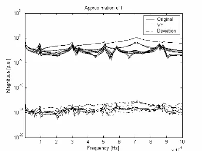
Fig. 2. Fitting of magnitudes by VF
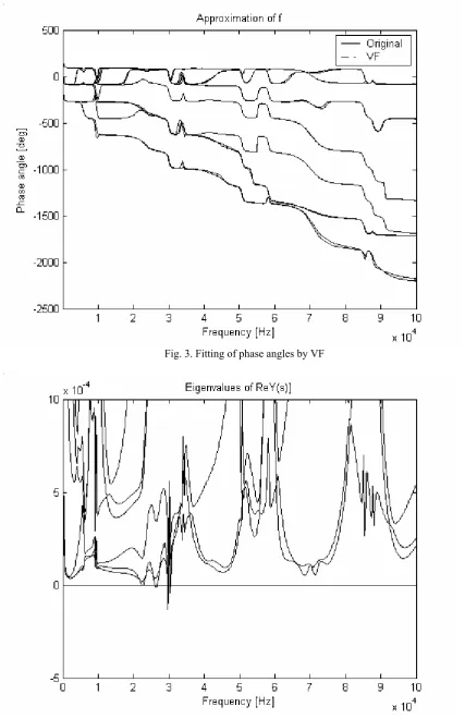
In this fitting process, 50 complex pair poles are selected as the initial poles. Figures 2 and 3 show the fitted magnitudes and phase angles of the elements of the 6×6 admittance matrix Ythrough an improved versionof VF [36].
Fig. 3. Fitting of phase angles by VF
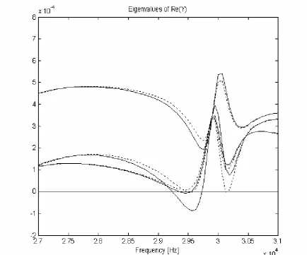
Fig. 5. Passivity enforcement via interior-point methods; solid curves: original model characteristics (before passivity enforcement), doted curves: model characteristics after perturbation
7. CONCLUSION
This paper demonstrates that optimization can be used to enforce the passivity of rational functions employed to approximate a power network (or components) equivalent. The method yields a globally optimal solution with minimum perturbation and a high degree of efficiency. The efficiency is achieved based on the utilization of the recently developed interior-point methods. In the application of this method, first the Hamiltonian matrix theory, which is a purely algebraic method, is employed to find the passivity violation regions. Then the global passivity is ensured by extending the inequality constraint, used in a convex optimization problem, to all the frequency points in the frequency range of approximation.
REFERENCES
1. Gustavsen, B. & Semlyen, A. (1999). Rational approximation of frequency domain responses by vector fitting.
IEEE Trans. Power Delivery, Vol. 14, No. 3, pp. 1052–61.
2. Gustavsen, B. & Semlyen, A. (1998). Application of vector fitting to the state equation representation of transformers for simulation of electromagnetic transients. IEEE Trans. Power Delivery, Vol. 13, No. 3, pp. 834-42.
4. Abdel-Rahman, M., Semlyen, A. & Iravani, M. R. (2003). Two-layer network equivalent for electromagnetic transients. IEEE Trans. Power Delivery, Vol. 18, No. 4, pp. 1328-35.
5. Gustavsen, B. (2004). Wide band modeling of power transformers. IEEE Trans. Power Delivery, Vol. 19, No. 1, pp. 414-22.
6. Ramirez, A., Naredo, J. L. & Moreno, P. (2005). Full frequency-dependent line model for electromagnetic transient simulation including lumped and distributed sources. IEEE Trans. Power Delivery, Vol. 20, No. 1, pp. 292-99.
7. Grivet-Talocia, S. (2004). Passivity enforcement via perturbation of Hamiltonian matrices. IEEE Trans. Circuit and Systems I: Regular Papers, Vol. 51, No. 9, pp. 1755-69.
8. Saraswat, D., Achar, R. & Nakhla, M. S. (2004). A fast algorithm and practical considerations for passive macromodeling of measured/simulated data. IEEE Trans. Advanced Packaging, Vol. 27, No. 1, pp. 57-70. 9. Porkar, B., Vakilian, M., Shahrtash, S. M. & Iravani, R. (2007). Passivity enforcement via residues perturbation
for admittance representation of power system components. Iranian Journal Science & Technology, Transaction B, Engineering, Vol. 31, No. B3, pp. 273-288.
10. Boyd, S., Balakrishnan, V. & Kabamba, P. (1989). A bisection method for computing the H_infinity-norm of a transfer matrix and related problems. Mathematics of Control, Signals, and Systems, Vol. 2, No. 3, pp. 207-19. 11. Gustavsen, B. & Semlyen, A. (2001). Enforcing passivity for admittance matrices approximated by rational
functions. IEEE Trans. Power Systems, Vol. 16, No. 1, pp. 97–104.
12. Hendrickx, W., Deschrijver, D. & Dhaene, T. (2004). Some remarks on the vector fitting iteration. Lect. Notes Comput. Sci., Post-Conference Proceedings of ECMI.
13. Sanathanan, C. & Koerner, J. (1968). Transfer function synthesis as a ratio of two complex polynomials. IEEE Trans. Automatic Control, Vol. 8, No. 1, pp. 56-8.
14. Deschrijver, D., Dhaene, T. (2005). Broadband macromodelling of passive components using orthonormal vector fitting. Electronic Letters, Vol. 41, No. 21.
15. IEEE Power Engineering Society, Tutorial on modern heuristic optimization techniques with applications to power systems.
16. von Neumann, J. (1947). On a maximization problem. Technical Report, Institute for Advanced Study (Princeton, NJ, USA).
17. Hoffman, A. J., Mannos, M., Sokolowsky, D. & Wiegman, N. (1953). Computational experience in solving linear programs. Journal of the Society for Industrial and Applied Mathematics, Vol. 1, pp. 17-33.
18. Frisch, K. R. (1955). The logarithmic potential method of convex programming. Technical report, University Institute of Economics, Oslo, Norway.
19. Karmarkar, N. K. (1984). A polynomial-time algorithm for linear programming. Combinatori-ca, Vol. 36, pp. 373-95.
20. Barnes, E. R. (1986). A variation on Karmarkar's algorithm for solving linear programming problems. Math. Programming, Vol. 36, pp. 174-82.
21. Gill, P. E. & Morray, W. (1986). On projected Newton barrier methods for linear programming and an equivalence to Karmarkar's projective method. Math. Programming, Vol. 36, pp. 183-209.
22. Marsten, R. E. & Saltzman, M. J. (1989). Implementation of a dual affine interior point algorithm for linear programming. ORSA Journal on Computing, Vol. 1, pp. 287-97.
23. Gonzaga, C. C. (1992). Path following methods for linear programming. SIAM Review, Vol. 34, pp. 167-224. 24. Wright, S. J. (1997). Primal-dual interior-point methods. SIAM.
25. Todd, M. (1995). Potential reduction methods in mathematical programming. Technical Report 1112, Cornell University, Ithaca, NY.
27. Roos, C., Terlaky, T. & Vial, J. (1996). Theory and algorithms for linear optimization: an interior point approach, John Wiley & Sons.
28. Nesterov, Y. & Nemirovskiy, A. (1994). Interior-point polynomial methods in convex programming. Society for Industrial and Applied Mathematics.
29. Nesterov, Y. E. & Todd, M. J. (1998). Primal-dual interior-point methods for selfscaled cones. SIAM Journal on Optimization, Vol. 8, No. 2, pp. 324-64.
30. Boyd, S. & Vandenberghe, L. (2004). Convex optimization. Cambridge University Press. 31. Ye, Y. (1997). Interior-point algorithm, theory and analysis. John Wiley & Sones. 32. BPMPD, [Online]. Available: http://www.pserc.cornell.edu/bpmpd/
33. Meszaros, C. (1996). The efficient implementation of interior point methods for linear programming and their applications. PhD Thesis, Eotvos Lonand University of Sciences, PhD School of Operations Research, Applied Mathematics and Statistics, Budapest, Hungary.
34. MATPOWER, [Online]. Available: http://www.pserc.cornell.edu/matpower/
35. Mehrotra, C. (1992). On the implementation of a primal-dual interior point method. SIAM Journal on Optimization, Vol. 2, pp. 575-601.