ROBUST OPTIMAL SPEED TRACKING
CONTROL OF A CURRENT SENSORLESS
SYNCHRONOUS RELUCTANCE MOTOR DRIVE
USING A NEW SLIDING MODE CONTROLLER
J. Soltani and H. Abootorabi Zarchi
Department of Electrical and Computer Engineering, Isfahan University of Technology Isfahan, Iran, [email protected] - [email protected]
(Received: October 14, 2003 - Accepted in Revised Form: February 26, 2004)
Abstract
This paper describes the robust optimal incremental motion control of a current sensorless synchronous reluctance motor (SynRM), which can be specified by any desired speed profile. The control scheme is a combination of conventional linear quadratic (LQ) feedback control method and sliding mode control (SMC). A novel sliding switching surface is employed first, that makes the states of the SynRM follow the nominal trajectories (controlled by any type of nominal controller) when the motor parameter uncertainties and the disturbance load torque exist. The SM controller has no reaching phase and produces small SMC chattering. Then, using the above tracking controller, the well-known torque control schemes, maximum torque (MTC), constant current inductive axis control (CCIAC) and maximum power factor control (MPFC) related to the SynRM are examined below and above the base speed. Finally the validity of our proposed control scheme is verified by computer simulation results.Key Words
Robust Optimal, Speed Tracking, SynRM, Sliding Mode, Controller
ﻩﺪﻴﻜﭼ
ﻩﺪﻴﻜﭼ
ﻩﺪﻴﻜﭼ
ﻩﺪﻴﻜﭼ
ﻪﻌﻄﻗﻪﺑﻪﻌﻄﻗﺖﮐﺮﺣﻡﻭﺎﻘﻣﻭﻪﻨﻴﻬﺑ ﻝﺮﺘﻨﮐﻪﻟﺎﻘﻣﻦﻳﺍ )
Incremental Motion (
ﻥﻭﺮﮑﻨﺳ ﺭﻮﺗﻮﻣﮏﻳ
ﯽﺴﻧﺎﺘﮑﻟﺭ (SynRM) ﯽﻣﺡﺮﺷﺍﺭﻩﺪﺷﻒﻳﺮﻌﺗﺖﻋﺮﺳﻪﺼﺨﺸﻣﮏﻳﺀﺍﺯﺍﺭﺩﺖﻋﺮﺳﺭﺍﺩﺮﺑﻪﻧﻮﻤﻧﻥﻭﺪﺑ
ﺪﻫﺩ . ﺵﻭﺭ
ﮏﺑﺪﻴﻓ ﺎﺑﯼﺯﺎﺳﯽﻄﺧ ﻝﺮﺘﻨﮐﯼﺎﻬﺷﻭﺭﺯﺍﯽﺒﻴﮐﺮﺗ ﻝﺮﺘﻨﮐ ﻪﺑ ﻡﻮﺳﻮﻣﺖﻟﺎﺣ
(LQ)
ﯽﺷﺰﻐﻟﺖﻟﺎﺣﻩﺪﻨﻨﮐﻝﺮﺘﻨﮐﻭ
ﻲﻣ ﺪﺷﺎﺑ .
ﯽﻣﻪﺘﻓﺮﮔ ﺭﺎﮑﺑ ﺪﻳﺪﺟ ﯽﺷﺰﻐﻟﺢﻄﺳﮏﻳ ﺍﺪﺘﺑﺍ ﺭﻮﺗﻮﻣﯽﻣﺎﻧﺖﻟﺎﺣ ﺮﻴﺴﻣ ﺐﻴﻘﻌﺗﻪﮐ ﺩﻮﺷ
(SynRM) ﺍﺭ
ﯽﻣﻢﻫﺍﺮﻓﺭﻭﺎﺘﺸﮔﺵﺎﺸﺘﻏﺍﻭﯼﺮﺘﻣﺍﺭﺎﭘﯼﺎﻫﯽﻨﻴﻌﻣﺎﻧﻪﺑﺖﺒﺴﻧ ﺩﺭﻭﺁ
. ﯽﮔﺪﻳﺭﻮﺷﯼﺍﺭﺍﺩﯽﺷﺰﻐﻟﯽﺒﻴﮐﺮﺗﻩﺪﻨﻨﮐﻝﺮﺘﻨﮐ
ﻥﺪﻴﺳﺭﺯﺎﻓﺪﻗﺎﻓ ﻭﻢﮐ ﯽﻣ
ﺪﺷﺎﺑ . ﺲﭙﺳ ﯼﺭﺍﺪﻫﺎﮕﻧﺖﺑﺎﺛ،ﺭﻭﺎﺘﺸﮔﻢﻤﻳﺰﮐﺎﻣﯽﻟﺮﺘﻨﮐﯼﺎﻫﺭﺎﮑﻫﺍﺭ،ﻩﺪﻨﻨﮐﻝﺮﺘﻨﮐﻦﻳﺍﺎﺑ
ﺭﻮﺗﻮﻣﻪﺑ ﻁﻮﺑﺮﻣ ﻥﺍﻮﺗ ﺐﻳﺮﺿ ﻢﻤﻳﺰﮐﺎﻣ ﻭ ﻢﻴﻘﺘﺴﻣﺭﻮﺤﻣ ﻥﺎﻳﺮﺟ SynRM
ﺮﻈﻧﺭﺩ ﻪﻳﺎﭘﺖﻋﺮﺳ ﯼﻻﺎﺑ ﻭ ﺮﻳﺯ ﺭﺩ
ﯽﻣﻪﺘﻓﺮﮔ ﺪﻧﻮﺷ .
ﺗﻮﻴﭙﻣﺎﮐﯼﺯﺎﺳﻪﻴﺒﺷﮏﻳﯽﻃ ﺎﻣﯼﺩﺎﻬﻨﺸﻴﭘ ﻝﺮﺘﻨﮐﺵﻭﺭﺖﺤﺻﻭﯼﺭﺍﺮﻗﺮﺑ،ﺖﻳﺎﻬﻧﺭﺩ ﺩﺭﻮﻣﯼﺮ
ﯽﻣﺭﺍﺮﻗﺶﻳﺎﻣﺯﺁ ﺩﺮﻴﮔ
.
1. INTRODUCTION
The high performance inverter-fed synchronous reluctance motor drive due to a number of its benefits such as simplicity of construction and control, high efficiency and low cost has attracted interest as an alternative for ac drive [1,2,3]. During the last two decades, many researchers have tried to present the more advanced control schemes by combining sliding mode control and fuzzy control [4,5]. Sliding mode variable structure control (SMVSC) has some favorable advantages, such as its insensitivity to parameter uncertainties and external disturbances. Only the bounds of the
Using this controller, simulation and experimental results were obtained for the control scheme maximum torque control (MTC) related to the SynRM.
In some control applications, such as robot, elevator and machine tool drives, it is needed to move a given load, stop it at a specified position and hold it there until a subsequent motion command is initiated. In such a condition, to make sure of moving the load to specified position at specified time, a desired velocity profile (most commonly the trapezoidal velocity profile) must be designed beforehand. This kind of start-stop motion is called the incremental motion control. Reference [7] has solved a particular incremental motion control problem, which is specified by a trapezoidal velocity profile. Using a multi-segment sliding mode control, each segment of the multi-segment switching surfaces has been derived to match the corresponding part of the trapezoidal velocity profile. To the best of our search, no more published paper or report was found which describes the speed tracking control of the SynRM. In our belief, the multi-segments SMC presented in [7] has the following disadvantages: 1) The controller cannot track any desired velocity profile except one described in [7].
2) The multi-segments SM controller of [7] has been developed based on the SynRM nominal system in order to track a specified trapezoidal velocity profile and therefore is not capable of making the SynRM states follow the nominal trajectories when the parameter uncertainties and the external load torque occur.
3) Simulation and experimental results presented in [7], show a large SMC chattering and high transient currents. These are almost produced by the multi-segments SMC, used in [7], that forces the SynRM nominal states on to the complicate and non-conventional sliding mode switching surfaces.
4) In [7], only the control strategy maximum torque (MTC) related to the SynRM was examined below the base speed. With reference to [3], the SynRM MTC strategy cannot be maintained as the load torque continues to increase since at some points the flux established in the direct axis begins to exceed its rated value.
To overcome the above problems, this paper presents the following control method for the rotor
speed and position tracking objectives of the SynRM.
i) The LQ feedback control method and SM control are combined to develop a new type of composite speed tracking controller for the SynRM perturbed system. A novel sliding surface is employed which is based on an augmented system whose dynamics have a higher order than that of the original system [8], the SynRM can be incremental motion controlled for any desired speed reference profile below and above the base speed. As a result, any type of controller, which is differentiable, can be a nominal controller. The composite controller has no reaching phase and produces small SMC chattering.
In the SynRM nominal system condition, the motor nominal trajectories always lie on the sliding surface and controlled by the LQ feedback control method. The LQ feedback controller, because is derived based on linear optimal control method, therefore it guarantees a perfect speed and rotor position tracking objectives for the SynRM nominal system.
In the perturbed system condition when the parameter uncertainties and disturbance load torque exist, an extra control effort is generated by the SM controller that forces the perturbed system trajectories on to the sliding surface or in other words makes them follow the system nominal trajectories.
ii) Control scheme maximum torque (MTC) related to the SynRM is selected first, and as the load torque begins to continues, this strategy is automatically changed into the constant current inductive axis control (CCIAC) scheme, followed by maximum power factor control (MPFC) strategy
iii) The estimated currents are used for the SynRM motion control. A current sensor less SynRM drive system has been described in [9] where the transient response of currents and the limitation of the inverter available voltage have not been taken in account. In the present current sensorless SynRM, the transient response of the
axes
dq
−
currents are arbitrarily designed while the constraint of the available voltage of the inverter is also taken into account.inverter used in [7], has less harmonic contents and in addition it provides a better utilization of the available dc link voltage. The remainder of this paper is organized as follows: in section II, the SynRM model and different torque control strategies related to this motor are explained. The SynRM currents estimation is described in section III and in section IV,
LQ
andSM controllers are explored. System simulation is show in section V and finally in section VI, conclusions are presented.2. SYNRM SYSTEM MODELING
With reference to [3], the rotor
ds
r−
qs
r:
axesequations for the SynRM are described by
r qs q e r ds s r ds d r
ds
R
i
L
i
dt
di
L
v
=
+
−
ω
(1)r ds d e r qs s r qs q r
qs
R
i
L
i
dt
di
L
v
=
+
+
ω
(2)r qs q r qs r
ds d r
ds
=
L
i
λ
=
L
i
λ
,
(3)where
v
dsr andv
qsr are theds
r−
qs
r:
axes statorvoltages,
i
dsr andi
qsr are the stator two axis currents,L
d andL
qdenote the SynRM inductances andω
e is the rotor electrical angular velocity. Also, the motor torque is) 2 sin( ) (
2 4
3 2
δ
s q d
e L L i
P
T = − (4)
where
P
is the number of stator poles,δ
is the angle of stator current vectori
s relative to the rotor d axis. In addition, the motor mechanical equations arel e m m m
m
B
T
T
dt
d
J
ω
+
ω
=
−
(5)m m
dt
d
ω
θ
=
(6)where
J
m is the rotor moment of inertia,B
m is the friction coefficient,θ
m is the rotor displacement angle in mechanical degrees,ω
m is the rotor angular velocity andT
l denotes the motor load torque.2.1 SynRM Torque Control Schemes
Ignoring the SynRM copper and iron losses, the torque control schemes related to this motor are described as follows [3]
a) MTC with
δ
=
45
o and 2s t
e
K
i
T
=
with
) (
2 4 3
q d
t L L
P
K = − (7)
b) CCIAC or
i
ds constant. c) MPFCwith
q d
L
L
1tan
−=
δ
(8)d) Maximum rate of change of torque (MRCTC) With
q d
L
L
1tan
−=
δ
(9)Using Equations 3-4, assuming the CCIAC control strategy, the SynRM torque equation is
r qs t
e
K
i
T
=
(10)The MTC strategy can not maintained as load torque continues to increase since at some points the flux established in thedaxis by
I
dsbegins to exceed the motor rated flux under the maximum power factor condition (rated condition).drated e
ds
ds
X
Then, the SynRM MTC scheme must be changed into CCIAC scheme while the
q
axis currentI
qs continues to increase until the MPFC strategy is reached based on the following equation.q d ds qs
L
L
I
I
=
(12)2.2 SynRM Field Weakening Mode Of
Operation
Because no interaction torque exists in a SynRM, therefore the field weakening in SynRMs is more difficult than a separately excited dc machine or a vector controlled induction motor drive. Nevertheless, a constant power characteristic can be achieved in the following way. Assume the stator flux linkage *)
(base
s
λ
at the base speed and under the SynRM maximum power factor (rated condition), therefore the stator flux linkage in the field weakening region for rotor speedω >
eω
b ise b base s s
ω
ω
λ
λ
* ) (*
=
(13)Reference [3] has shown that the maximum field weakening range for constant stator flux of the
SynRM is described by:
) (
2 1
d q q
d b
e
L L L
L
+ <
ω
ω (14)
Also, in sinusoidal steady-state condition
2 2
2 2
2
)
( r
qs r
ds q d
q
s I I
X X X
V
+
= (15)
From Equation 15, for the motor constant torque mode of operation
b e sb
b e
s V for
V ω <ω
ω ω
= . (16)
And in the field weakening region
b e sb
s V for
V = ω ≥ω (17)
Linking Equations 15 and 17, it yields
2 2 2 2
2
2 .( ) ( )
1 r
qs r
ds q d q
b sb
e b
I I L L L
V
+ =
ω
ω ω
(18)
q-axis
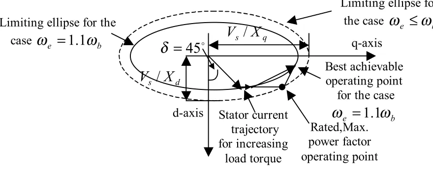
d-axis
Limiting ellipse for the
case
ω
e=
1
.
1
ω
bLimiting ellipse for
the case
ω
e≤
ω
bStator current
trajectory
for increasing
load torque
Rated,Max.
power factor
operating point
Best achievable
operating point
for the case
b
e
ω
ω
=
1
.
1
o
45
=
δ
V
s/
X
qd
s
X
V
/
Equation 18 explains an ellipse on the
d
−
q
plane with the major axis on theq
−
axis and minor axis on the d axis. Figure 1 shows that the size of this ellipse begins to decrease inversely with the square of the frequency ratio
b e ω
ω .
Assuming that the maximum current amplitude must remain fixed at the value defined by the base or rated condition, fixes the range of operation on the ellipse for any frequency.
In this case, the maximum current for each speed is chosen as that value, which will produce the SynRM rated power.
3. SYNRM CURRENTS ESTIMATION
Using Equations 1-2, the motor currents are
estimated as:
) v~ ( ) R S L
1 ( ) v v ( ) R S L
1 (
iˆ d
s d 0 d r * ds s d ds
+ = − +
=
(19)
) ~ ( ) 1 ( ) (
) 1 ( ˆ
0 *
q s q q
r qs s q
qs v
R S L v
v R S L i
+ = − +
=
(20)
ds ds q
qs qs
d
L
i
v
L
i
v
0=
−
ω
ˆ
,
0=
ω
ˆ
(21)where
v
ds*r and r qsv
* are d-axis and q-axis components of the PWM inverter voltage reference command.~
i
ds and~
i
qs currents are used for the SynRM motion control. Equations 19 and 20 arePI
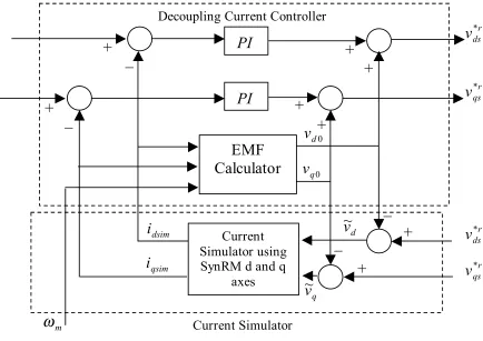
PI
Current Simulator
Decoupling Current Controller
r ds
v
*r qs
v
*r ds
v
*r qs
v
* dsimi
qsim
i
d
v
~
q
v
~
0 d
v
0 q
v
Current
Simulator using
SynRM d and q
axes
EMF
Calculator
+
_
+
_
+
+
+
+
+
_
+
_
m
ω
implemented in a current simulator as shown in Figure 2.
In Figure 2, the voltages
v
~
d andv
~
q are the output signals of two conventionalPI
current controllers, which are described in Section 6. From Figure 2, one can see that the reference voltagesv
ds*r and rqs
v
* are used to estimate the SynRM currents. In the other hand, in a two level three-phase SV-based PWM inverter [10]2 * 2 * ) ( ) ( . . 2 3 r qs r ds dc
ref m V v v
V = = + (22)
where m is the modulation index andVdcand
V
ref are respectively the dc link and the inverter reference voltages. From Equations 19-22, it can be concluded that in the current estimator of Figure 2, the transient state of the motor currents and the limitation of the inverter available voltage are simultaneously taken into account4. ROTOR SPEED TRACKING CONTROLLER
4.1 Nominal Control Input
A robust optimal speed tracking control is derived for the SynRM perturbed system in the following way. The tracking controller is robust and stable subject to the parameter uncertainties and the external load torque. Using Equations 4, 5 and 6, the mechanical state-space model of the SynRM in canonical form is: l m e m m m m m m mT
J
1
0
T
J
1
0
J
B
0
1
0
−
+
ω
θ
−
=
ω
θ
&
&
(23) Assume thatθ
ref andω
ref respectively are therotor speed and position reference commands, then the deviation form of Equation 23 becomes
)
(
t
Df
Bu
Ax
x
&
=
+
+
(24)where
)
t
(
f
),
2
sin(
i
)
t
(
u
,
b
0
B
,
a
0
1
0
A
=
s2δ
=
−
=
),
a
T
(
L′
+
ω
d+
ω
d=
&
(25)
ω
−
ω
=
θ
−
θ
=
=
=
ref m 2 ref m 1 2 1x
x
,
x
x
x
,
1
0
D
with reference to [6], the linear quadratic feedback control method (LQ) is easily able to achieve the dynamic system requirement for a linear control system. Consider Equation 24, the performance index for the SynRM nominal system is
∫
∞+
=
0 2 0 0 01
(
)
2
1
dt
u
r
x
Q
x
J
T (26)where
r
is a positive constant andQ
is a positive definite matrix. The choice of elements of matrixQ
and positive constantr
must take the physical condition for the motor system in to consideration. Usually, the smallerr
is, the larger the control feed back and control law will be. By introducing a co-state variable vectorP
, the SynRM state model of (24) and the cost function (26) are appended to form the following Hamiltonian generalized co-energy function.]
[
]
[
2
1
0 0 2 0 00
Qx
r
u
P
Ax
Bu
x
H
T T+
+
+
=
(27)Applying Pontryagin’s maximum principle [11], to Equation 27, defining the vector P as
x S
P = (28)
where
S
is the solution of the Riccatee equation0 1
= + −
+ SBB S Q
r SA S
AT T (29)
)
(
)
(
)
,
(
0 0*
0
S
x
t
K
x
t
r
B
t
x
u
=
−
T=
−
T (30)where
K
is the vector of gains.4.2. Curbing Control Input
In the perturbed system condition, steady-state error would exist if the drive system control were derived based on the LQ feedback control method. In such a condition, the SynRM system model isp bu
Ax
x& = + + ~ (31) where
p
~
is the lumped uncertainty and is definedby
) (
~p = ∆Ax + ∆B u + Df t (32)
To conserve the responses and reject the effects of the external disturbance and parameter uncertainties, a sliding mode controller with a new sliding switching surface is developed [8]. The sliding surface is derived based on an augmented system, which has a virtual state. The virtual state is obtained from the controllable canonical form of the nominal system. Consider the controllable canonical form of the nth-order system as
)
(
)
(
)
(
)
(
)
(
)
(
t
A
A
x
t
B
B
u
t
Df
t
x
=
+
∆
+
+
∆
+
(33) where = − − − = 1 . . 0 , . . . . . . . . . . 0 1 0 0 . . . 0 1 0 2 1 B A n α α α (34)
where
x
∈
R
n,
u
∈
R
,
f
∈
R
r and the boundeduncertainties
∆
A
,
∆
B
and the disturbance matrixD
satisfying the following matching conditionB
rank
D
B
A
B
rank
[
:
∆
:
∆
:
]
=
(35)The novel virtual state is described by
n n
n v n
v
x
t
x
t
u
x
t
x
x
=
−
(
)
−
−(
)
−
⋅
⋅⋅
+
&
(
,
)
=
&
~
0 0 1
α
α
(36)where
)
,
(
00
x
t
u
is a nominal regulating control input and differentiable .For this augmented system, the sliding surface is chosen as)
t
,
x
(
u
)
t
(
x
)
t
(
x
)
t
(
x
)
t
(
x
S
1 1 1 n 1 n n n v−
α
+
⋅
⋅
⋅
+
α
+
α
+
=
− − (37)where
u
(
t
)
is the SMC control input that guaranties the sliding mode on the sliding surface . Using Equation 24, the virtual state and the augmented system for the SynRM is obtained as + − − = + ∆ + + ∆ + = ) ( ~ ) ( ) ( ) ( ) ( ) ( ) ( 0 2 2 1
1x a x u x
a x t f D t u B B t x A A t x & & & (38)
From Equation 37, the novel sliding surface, is given by
)
(
~
)
,
(
x
t
x
a
1x
1a
2x
2u
0x
S
=
+
+
−
(39)where
u
&
0(
t
)
is obtained by the derivative of (30) with respect to time t.x
L
x
K
B
Ax
K
x
u
B
Ax
K
t
x
K
t
u
T T T T−
=
−
−
=
+
−
=
−
=
)
(
))
(
(
)
(
)
(
0 00
&
(40) with)
(
TT
A
B
K
K
L
=
−
(41)With reference to Equation 36, the virtual state x~ must be chosen as
2
~
x
x
=
&
(42)To force the system states curb on to the novel sliding surface, the SM reaching condition must be satisfied by:
0
)
~
,
(
)
~
,
(
x
x
S
x
x
<
S
&
(43)With reference to [8], using Equations 25 and 39-42, the following input guaranties the validity of Equation 43.
)
S
sgn(
)
|
)
t
(
u
|
||
)
t
(
x
||
(
B
)
K
C
((
))
t
(
Ax
)
K
C
(
Lx
x
(
B
)
K
C
((
)
t
(
u
3 2 1 1 1 1 1 2 2 1 1γ
+
γ
+
γ
+
−
+
+
+
α
−
+
−
=
− −&
(44) where]
,
0
[
1a
C
=
−
(45)And
γ
1,
γ
2 andγ
3 are the positive constants satisfying the following conditions:||
)
(
||
)
(
)
(
C
1+
K
∆
A
x
t
<
γ
1x
t
(46)|
)
(
|
)
(
)
(
C
1+
K
∆
B
Ux
t
<
γ
2u
t
(47)3
1
)
(
)
(
C
+
K
Df
t
<
γ
(48)In order to reduce the SMC chattering, one easy solution may be replacing the sign function,
)
sgn(
S
, by a boundary layer saturation function as [12]. ϕ − < − ϕ ≤ ϕ ϕ > = ϕ S if S if S S if S sat 1 1 )( (49)
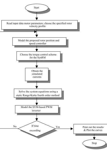
5. SYSTEM SIMULATION
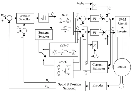
Block diagram of Figure 3 is proposed for rotor speed and position tracking objectives of the
current sensorless SynRM drive system. This figure shows that the supply voltage of the motor is synthesized from the stator
d
r−
q
r:
axes voltagecommands
(
*,
*)
qs dsv
v
, using a two level space vector modulation SVM-based PWM inverter. In addition, this figure also shows that as the load torque continues to increase, the torque control schemes MTC, CCIAC and MPFC related to the SynRM are automatically selected. Moreover, a current estimator is also used to detect the motor currents. Furthermore, the rotor speed and position are sampled by high-resolution digital sensors.A
C
++step-by-step computer language program was developed to model the drive system control of Figure 4. In this program, the system dynamic equations are solved using a static Runge-Kutta fourth order method. Variable to solve for arei
ds,
i
qs,
θ
randω
r. Flow chart of this program is illustrated in Figure 4.Computer simulation results obtained for a SynRM with parameters shown in Tab.1. Using these parameters, the LQ feedback controller gains were calculated as:
T
K
=
[
31
.
68
,
31
.
62
]
for
=
100
0
0
100
Q
(50)and r =0.1
of Figures 5 and 6, but with J=5Jn applied at 4 sec, a simulation test was also carried out to demonstrate the SynRM performance below and
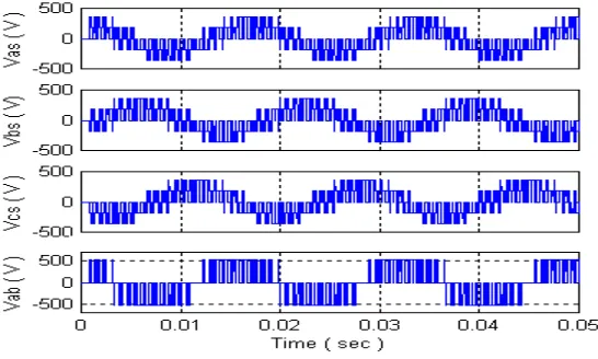
above the base speed. The results of this test are shown in Figures 7 and 8. In addition, the PWM inverter simulated results are given in Figure 9.
Combined Controller
r s i
r qs i r ds i
MTC
* 2
2 | * | *
= =
2 * 2 * ( | *
|iqsr isr idsr CCIAC
− =
MPFC
q L
d L r ds i
r qs i
=
* *
Strategy Selector
PI
PI
SVM Circuit
& Inverter
SynRM
Encoder Speed & Position
Sampling
Current Estimator
ref
ω
ref
θ
u
r s
i* r
ds
i*
r qs
i*
q mL
ω
d mL
ω
r ds
v*
r qs
v*
r ds
iˆ
r qs
iˆ
m
θ
m
ω
d
v
~
q
v
~ +
_
+ _
+ _
+ _
+ + +
_
Figure 3.Block diagram of SynRM drive system control.
TABLE 1.SynRM Parameters.
n
P
1120
W
r
s0
.
91
Ω
J
m 0.01Kgm
2n
V
230
V
L
ds135
mH
B
m0
.
002
N
.
m
.
s
n
f
60
Hz
L
qs50
mH
r
r≅
0
Ω
P
4
poles
n
I
6
.
6
A
TABLE 2.Coefficients of the Conventional PI Controllers and the Proposed SMC.
The coefficients of the proposed SMC
1
.
5
1
=
γ
γ
2=
90
γ
3=
8000
The coefficients of PI controllers
=
320
P
Start
Read input data motor parameters; choose the specified rotor velocity profile
Model the proposed rotor position and speed controller
Choose the torque control scheme for the SynRM
Obtain the simulated currents
Solve the system equations using a
-static Range-Kutta fourth order method
Model the SVM-based PWM inverter
Print out the results & Plot the curves
Stop
No If time Yes
exceeding
6. DISCUSSION
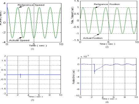
With reference to Figure 5 (2), the steady-state error that exists in the SynRM rotor position is because of the LQ feedback controller, which is not robust to the system uncertainties and the external disturbance. From simulated results shown in Figures 6 and 8, one can conclude that the proposed tracking controller is capable of making in the SynRM perturbed system states follow the nominal system trajectories. The high frequency oscillations seen on these figures are produced by the inverter harmonics as well as by the SMC small chattering. In addition, in Figures 6 (3) and 8 (3), the notches are caused by the step changes that exist in the motor acceleration and load torque
reference commands. Furthermore, from Figures 7 (2) and 7 (3) or Figures 8 (8) and 8 (9), it is seen that the SynRM drive system, initially operates in its MTC scheme and as the load torque continues to increase, this strategy is automatically changed into the CCIAS and MPF control schemes related to this motor.
7. CONCLUSIONS
Robust optimal speed and position tracking control of a current sensorless SynRM drive system has been described. The torque control schemes, MTC, CCIAC and MPFC related to SynRM has been
(1) (2)
(3) (4)
Figure 5.SynRM speed tracking control assuming a sinusoidal velocity profileusing the LQ controller:
examined below and above the base speed. The LQ feedback control method and SM control method have been combined to develop a new type of the rotor speed and position tracking controller for the SynRM perturbed system The composite controller employs a novel third order sliding surface that makes the motor perturbed system states follow the nominal trajectories. The nominal trajectories are controlled by the LQ feedback control method. The novel SM controller has no reaching phase and produces a small SMC chattering.
The specified sinusoidal and trapezoidal speed reference profiles were tested by digital simulation. Computer simulation results obtained, confirm the effectiveness of the proposed control method. A current estimator has also been presented in which
the motor current transient states and the limitation of the inverter available voltage are s taken into account simultaneously.
8. REFERENCES
1. Lipo, T. A. ,"Synchronous Reluctance Machines A Viable Alternative for Ac Drives", Electric Machines and Power Systems, Vol. 19, (1991), 659-671.
2. Boldea, I., Muntean, N. and Nasser, S. A., ”Robust Low-Cost Implementation of Vector Control for Reluctance Synchronous Machines”, IEE Proc.- Elect. Power Appl., Vol. 141, Issue 1, (January 1994), 1-6.
3. Matsuo, T. and Lipo, T. A., ”Field Oriented of Synchronous Reluctance Machine”, IEEE, IA-33, (1993), 1146-1153.
(1) (2)
(3)
(4)
Figure 6. SynRM incremental motion control assuming a sinusoidal velocity profile using the proposed composite SMC (1) Rotor speed with composite SMC, (2) Rotor position with composite SMC, (3) Rotor speed error with composite SMC and
(1) (2) (3)
(4) (5)
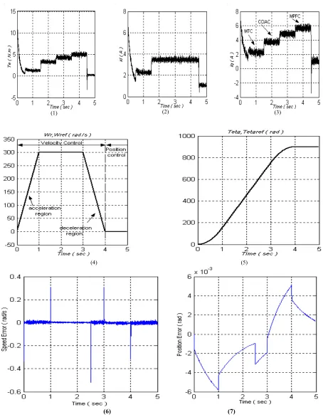
(6) (7)
Figure 7. SynRM incremental motion control below the base speed, assuming a specified trapezoidal velocity profile using the composite SMC: (1) Motor torque, (2) Stator d axis current, (3) Stator q axis current, (4) Rotor speed,
(1)
0 2 4 6 8 10
-200 0 200 400 600 800 1000 1200 1400
Time ( sec )
Te
ta
,T
et
ar
ef
(
r
a
d
)
(2)
(3) (4)
(5) (6)
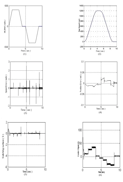
Figure 8. SynRM incremental motion control above the base speed, assuming a specified trapezoidal velocity profile using the composite SMC: (1) Rotor Speed, (2) Rotor Position, Speed error (rad/s), (4) Position error (rad/s), (5) Sliding function and
4. Liu, T. H. and Lin, M. T., "Fuzzy Sliding-Mode Controller Design for a Synchronous Reluctance Motor Drive", IEEE Trans. On Aerospace and Electronic Systems, Vol. 32, No. 3, (July 1996), 1065-1076.
5. Wai, R. J., “Adaptive Sliding-Mode Control for Induction Servomotor Drive”, IEE Proc. Electr. Power Appl., Vol. 147, No. 6, (November 2000), 553-562. 6. Shyu, K. K., Lai, C. K. and Tsai, Y. W., “Optimal
Position Control of Synchronous Reluctance Motor via Totally Invariant Variable Structure Control’’, IEE Proc. Control Theory Appl., Vol. 147, No. 1, (January 2000, 28-36.
7. Shyu, Kuo-Kai and Lai, Chui-Keng, “Incremental Motion Control of Synchronous Reluctance Motor via Multisegment Sliding Mode Control Method”,
IEEE Trans. On Control Systems Technology, Vol. 10, No. 2, (March 2002), 169-176.
8. Park, S. K., and Ahn, H. K., “Robust Controller Design with Novel Sliding Surface’’, IEE Proc. - Control Theory Appl., Vol. 146, No. 3, (May 1999), 242-246.
9. Matsuo T. and Lipo T. A., IEEE IAS Ann. Meet., (1993), 672-678
10. Divan, D. M. and Lipo, T. A., “PWM Techniques for
0 5 10
-6 -4 -2 0 2 4 6 8
Time ( sec )
Te
(
N
.m
)
0 5 10
-8 -6 -4 -2 00 2 4 6
Time ( sec )
iq
(
A
)
0 5 10
0 1 2 3 4 5
Time ( sec )
id
(
A
) MTC
CCIAC MPFC
(7) (8) (9)
Figure 8 (continued from previous page). SynRM incremental motion control above the base speed, assuming a specified trapezoidal velocity profile using the composite SMC: (7) Motor torque,
(8) Stator q axis current and (9) Stator d axis current.
Voltage Source Inverters’’, Tutorial Notes, IEEE/PESC, San Antonio, (1990), 324-330.
11. Anderson, B. D. O. and Moore, J. B., “Linear Optimal
Control”, Prentice-Hall, (1971).