OPTIMUM AGGREGATE INVENTORY FOR SCHEDULING
MULTI-PRODUCT SINGLE MACHINE SYSTEM WITH
ZERO SETUP TIME
Alireza Haji and Rasoul Haji
Department of Industrial Engineering, Sharif University of Technology Tehran, Iran, [email protected] - [email protected]
(Received: April 9, 2001 – Accepted in Revised Form: August 20, 2001)
Abstract In this paper we adopt the common cycle approach to economic lot scheduling problem and minimize the maximum aggregate inventory. We allow the occurrence of the idle times between any two consecutive products and consider limited capital for investment in inventory. We assume the setup times are negligible. To achieve the optimal investment in inventory we first find the idle times which minimize the maximum aggregate inventory for a given sequence of production runs and for any arbitrary cycle time T . Then, we show that these values of idle times, for the given sequence, are also optimal idle times for any other sequence. The result is an easy-to-apply rule that greatly simplifies the task of scheduling to achieve minimum required investment in inventory.
ﻩﺪﻴﻜﭼ
ﻱﺩﻮﺟﻮﻣﺮﺜﻛﺍﺪﺣ ،ﻱﺍﻪﺘﺳﺩ ﻱﺩﺎﺼﺘﻗﺍ ﻱﺰﻳﺭ ﻪﻣﺎﻧﺮﺑ ﻪﻟﺎﺴﻣ ﻱﺍﺮﺑ ﻙﺮﺘﺸﻣﺭﻭﺩ ﺵﻭﺭﺎﺑ ﻪﻟﺎﻘﻣ ﻦﻳﺍ ﺭﺩﻮﺼﺤﻣ ﻲﻌﻤﺟ
ﺖﺳﺍ ﻩﺪﺷ ﻪﻨﻴﻤﻛ ﺕﻻ .
ﺖﻳﺩﻭﺪﺤﻣ ﻭﺕﻻﻮﺼﺤﻣ ﻦﻴﺑ ﺭﺩﻦﻴﺷﺎﻣ ﻱﺭﺎﻜﻴﺑ ﻱﺎﻬﻧﺎﻣﺯ ﻖﻴﻘﺤﺗﻦﻳﺍ ﺭﺩ
ﺖﺳﺍﺮﻔﺻ ﻱﺯﺎﺳﻩﺩﺎﻣﺁﻱﺎﻬﻧﺎﻣﺯ ﻪﻛﺖﺳﺍﻩﺪﺷﺽﺮﻓ ﻭﻩﺪﺷﻪﺘﻓﺮﮔﺮﻈﻧﺭﺩﻱﺩﻮﺟﻮﻣ ﺭﺩﺮﻴﮔﺭﺩﻪﻳﺎﻣﺮﺳ .
ﻱﺍﺮﺑ
ﺟﻮﻣﺮﺜﻛﺍﺪﺣﻱﺍﺮﺑﻱﺭﺎﻜﻴﺑ ﻱﺎﻬﻧﺎﻣﺯﺮﻳﺩﺎﻘﻣ ﺍﺪﺘﺑﺍ،ﻱﺩﻮﺟﻮﻣﺭﺩﺮﻴﮔﺭﺩﻪﻳﺎﻣﺮﺳﻪﻨﻴﻬﺑ ﺭﺍﺪﻘﻣﻦﻴﻴﻌﺗ ﺭﺩﻲﻌﻤﺟﻱﺩﻮ
ﻮﻠﻌﻣ ﻲﻟﺍﻮﺗ ﻚﻳ ﻡ
ﺖﺳﺍ ﻩﺪﻣﺁﺖﺳﺪﺑ ﻱﺭﺎﻴﺘﺧﺍ ﺪﻴﻟﻮﺗﺭﻭﺩ ﻚﻳ ﻭﺪﻴﻟﻮﺗ .
ﻪﻨﻴﻬﺑ ﺮﻳﺩﺎﻘﻣ ﻪﻛ ﻩﺪﺷﻩﺩﺍﺩ ﻥﺎﺸﻧ ،ﺲﭙﺳ
ﺩﺭﺍﺪﻧ ﻲﮕﺘﺴﺑ ﺪﻴﻟﻮﺗ ﻲﻟﺍﻮﺗ ﻪﺑ ،ﻱﺭﺎﻜﻴﺑ ﻱﺎﻬﻧﺎﻣﺯ .
ﺪﻫﺩ ﻲﻣ ﻪﺋﺍﺭﺍ ﻱﺩﺮﺑﺭﺎﻛ ﻥﺎﺳﺁ ﻩﺪﻋﺎﻗ ﻚﻳ ﻖﻴﻘﺤﺗ ﻦﻳﺍ ﻪﺠﻴﺘﻧ
ﻪﻳﺎﻣﺮﺳﻪﻨﻴﻤﻛﻪﺑ ﻞﻴﻧﻱﺍﺮﺑ ﺍﺭﻱﺰﻳﺭﻪﻣﺎﻧﺮﺑ ﺭﺎﻛ ﻪﻛﻱﺭﻮﻃ ﻪﺑ
ﻩﺩﺎﺳﻲﻬﺟﻮﺗﻞﺑﺎﻗﺭﻮﻃﻪﺑﻱﺩﻮﺟﻮﻣﺭﺩﺯﺎﻴﻧﺩﺭﻮﻣ
ﺩﺯﺎﺳﻲﻣ .
INTRODUCTION
The Economic Lot Scheduling Problem (ELSP) arises frequently in industry and research. The problem is to economically schedule lots (i.e., product runs) of one or more products on one multipurpose machine. The problem of determining economic production quantity (EPQ) for the case of one product is well known. However, in the case of two or more products, treating each item as independent does not work. For, in general, the economic production quantities so determined can not be feasibly scheduled, and the phenomenon of interference will occur sooner or later- that is the facility will be required to produce more than one item at the same time which is physically impossible [9].
There is no universal solution procedure available
which solves this problem optimally. This NP- hard problem is notoriously difficult to solve [3,10]. Several different types of approaches, either analytical approach to a restricted problem or heuristic approaches to the entire problem, have been presented in the literature (See, for instance, [1,4,5,13]).
In this research we adopt the CC approach and consider the importance of limited resources in managing the aggregate inventory of a multi-product single machine system. In a real-word situation, due to various reasons such as corporate policy or limitation on amount insured, the resources (e.g., capital or space) are limited. Parsons [12], Haji [6], and Haji and Mansouri [7] have considered the total investment in inventory in CC approach. But Parsons’ method unrealistically assumes the aggregate inventory is equal to the sum of the values of individual product lot sizes. In fact, in practice, the maximum aggregate inventory must be evaluated based on the sequence in which the products are produced and the amount of idle times allocated between consecutive products. Haji [6], and Haji and Mansouri [7], in their papers consider the sequence in which the products are produced in the cycle; but they impose the restriction that the total idle time in a cycle extends from the end of production run of the last product produced in the cycle up to the start of the next cycle where the production of the first product of the next cycle starts.
In this paper we consider limited investment and relax the above restriction, i. e., we allow the occurrence of idle time between production of any two consecutive products. This can provide some flexibility for performing certain tasks such as preventive maintenance. Also it may provide operators more rest times resulting in lower number of accidents and higher quality products. Then assuming the setup time is zero we minimize the maximum aggregate inventory for any common cycle time T (including optimal cycle time). To do this, we first develop a simple and easy- to- apply rule that finds the values of idle times which minimizes the maximum aggregate inventory for a given sequence of production runs of products and for any arbitrary cycle time T. Then, we show that these values of idle times for the given sequence are also optimal for any other sequence. That is, optimal idle times, and therefore, the corresponding optimal investment in inventory is independent of the production sequence.
MINIMIZATION OF MAXIMUM AGGREGATE INVENTORY
In this paper, all the standard assumptions of the
general ELSP hold true. The most relevant of the assumptions used in this paper are as follows:
1. There are N products, all of which must be
produced on a single machine. Machine can make only one product at the time.
2. Demand rates for all products are constant, known, and finite.
3. Production rates for all products are constant, known, and finite.
4. The time horizon is infinite.
5. All demands must be filled immediately. So, no shortages are permitted.
In addition, we consider the CC Scheduling approach, which implies:
6. In each common cycle, T, all of the products
will be produced.
7. Each product is produced only once in each
cycle T.
Furthermore it is assumed that:
8. During the production time of any product, the
aggregate inventory increases. That is, the production rate of any product (in units of money per unit time) is greater than the aggregate demand rate (in units of money per unit time).
The following notations are used in this paper: N Number of products.
Pj: Production rate of product j, in units of money
per time unit.
Dj Demand rate of product j, in units of money
per time unit.
D Aggregate demand in units of money per time unit (
∑
= N
1 j j
D
).T Common cycle time in units of time.
tj Production run-time of product j, j=1,2,…N.
Xj Duration of idle time occurring just before the
production run of product j, j=1,2,…N.
Ej Aggregate inventory in units of money at the
end of production run of product j, j=1,2,…N. Ij(t) Inventory level of product j at time t, in units
of money.
Imax Maximum aggregate inventory in units of
money.
Following the above notation, Imax can be
written as:
∑
≤ ≤
=
max
I
(
t
)
I
jT t 0 max
The value of Imax depends on the order of the
AGGREGATE INVENTORY AT THE END OF A PRODUCTION RUN
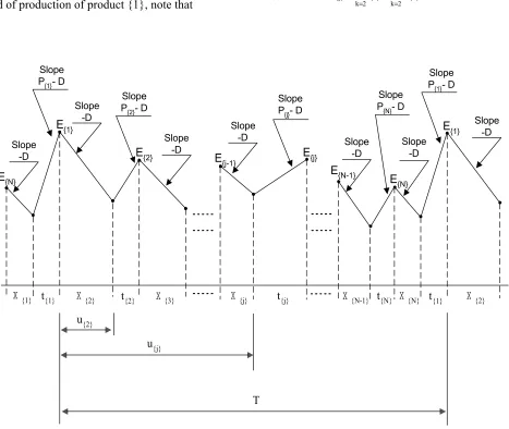
Consider an arbitrary production schedule of N products, which repeats itself every T time units. Choose a cycle T that begins just at the start of the production run of a particular product and ends at the start of the next production run of the same product.
Now designate the given sequence by {1},{2},…,{N}, where {1} represents the particular product and {j} represent the product that has j-th position in the sequence. In each cycle time T the aggregate inventory increases at the rate (P{j} –D) during t{j}
and decreases at the rate D during X{j}, j = 1, 2, …,
N, Figure 1.
To find E{j}, the aggregate inventory level at the
end of production of product {1}, note that
∑
=
=
N 1k {k}
} 1
{
I
E
(1)where
I{k} = the inventory level of product {k} at the end
of production run of product {1}, k=1,2,…, N. Clearly
} 1 { } 1 { } 1 { } 1
{
(
P
D
)
t
I
=
−
(2)To find I{j} , j ≥ 2, let u{j} = the length of time from
the end of production run of product {1} to the start of production run of product {j}, Figure 1. Thus
} 2 { } 2
{ X
u = , ∑− ∑
= + =
= j1
2 k
j
2 k {k} }
k { } j
{ t X
u .
Slope -D
Slope
-D Slope
-D
Slope -D
Slope -D Slope
-D
Slope -D
Slope P{1}- D
Slope
P{2}- D SlopeP
{j}- D
Slope P{N}- D
Slope P{1}- D
X{1} t{1} X {2} t{2} X{3} X{j} t{j} X{N-1} t{N} X{N} t{1} X {2}
u{j}
T
E{1}
E{2} E
{j-1} E{j}
E{N-1}
E{N}
E{1}
E{N}
u{2}
Since no shortage is permitted, I{j}, the inventory
level of product {j} at the end of production of product {1}, is equal to demand for that product during u{j}, j=1,2,…,N. That is, I{j} =D{j}u{j}.
Hence, for j = 2
} 2 { } 2 { } 2
{
D
X
I
=
j = 2 (3)and for j ≥ 3
∑ ∑ = − = + = j 2 i 1 j 2 i {i} } j { } i { } j { } j
{ D X D t
I j ≥ 3
or equivalently adding and subtracting D{j} t{j} , we
can write: } j { } j { j 2 i j 2 i {i} } j { } i { } j { } j
{ D X D t D t
I = ∑ + ∑ −
= =
j ≥ 2 (4)
The aggregate inventory at the end of production run of product {1}, form relations (1), (2), and {4), is
∑
∑
∑
= = =
+
−
+
−
=
N 2j {j} {j}
j
2 i
j
2
i {i}
} j { } i { } j { } 1 { } 1 { } 1 { } 1 {
t
D
t
D
X
D
t
)
D
P
(
E
(5)Since the aggregate inventory decreases at the rate D during X{j} and increases at the rate (P{j} –
D) during t{j}, j=1, 2, …, N, we can write for j =2
} 2 { } 2 { } 2 { } 1 { } 2
{
E
DX
(
P
D
)
t
E
=
−
+
−
j = 2 (6)and for all j ≥ 2
∑ ∑ = = + − − = j 2
k {k} {k} j
2 k {k} }
1 { } j
{ E D X (P D)t
E j ≥ 2 (7)
Lemma 1
For a given schedule and known X{j},j = 1, 2, …, N, if we decrease X{2} by an amount y,
increase X{3} by the same amount, and fix all other
X{j}, (j ≠ 2and 3), then,
(i) E{j}, (j ≠ 2) will decrease by D{2}y
and
(ii) E{2} will increase by (D - D{2})y
Proof
To prove (i) denote the new value of X
{j} byX’{j}, thus:
≠
∀
=
′
+
=
′
−
=
′
3
and
2
j
X
X
y
X
X
y
X
X
} j { } j { } 3 { } 3 ( } 2 { } 2 { (8) Clearly, } 3 { } 2 { } 3 { } 2{ X X X
X′ + ′ = + (8a)
and
∑
∑
= =′
=
j 2i {i}
j 2
i
X
{i}X
j
≥
3
(8b)
Now we denote the new value of the inventory of product {j}, at the end of production run of product {1}, by I’{j} j
= 1,2,…, N. Then, as we derived (2) and (3), we can write } 1 { } 1 { } 1 { } 1
{
(
P
D
)
t
I
′
=
−
j = 1
(9a) which implies } 1 { } 1 {I
I
′
=
and } 2 { } 2 { } 2
{
D
X
I
′
=
′
or from (3) and (8)
)
y
X
(
D
I
{′
2}=
{2} {2}−
(9b)which implies
y
D
I
I
{′
2}=
{2}−
{2}, j = 2 and, as we derived (4),
} j { } j { j 2 i j 2 i {i} } j { } i { } j { } j
{ D X D t D t
I = ∑ ′ + ∑ −
= =
j
≥
2
and from (4), and (8b)
} j { } j {
I
the end of production run of product {j}. Then,
∑
=
′
=
′
N1 j (j) )
1
(
I
E
and from (9a), (9b), and (9c), we can write
y
D
I
E
N {2}1 j {j} }
1
{
=
−
′
∑
=
or from (1), we have
y
D
E
E
{′
1}=
{1}−
{2} (10)To find E’{j} for j ≥ 2, as we derived (7), we can
write
∑ ∑
=
= ′ + −
− ′ =
′ j
2
k {k} {k} j
2 k {k} }
1 { } j
{ E D X (P D)t
E
j
≥
2(11)
Thus, for j ≥ 3, from (8b) and (10), we can write (11) as
∑ ∑= + = − −
− =
′ j
2
k {k} {k} j
2 k {k} }
2 { } 1 { } j
{ (E D y) D X (P D)t
E
, j
≥
3
or from (7)
y
D
E
E
{′
j}=
{j}−
{2}j
≥
3 , y >0
(12) which proves the part (i) of the lemma.To prove part (ii), note that for j = 2, from (11) we have
} 2 { } 2 { } 2 { } 1 { } 2
{
E
D
X
(
P
D
)
t
E
′
=
′
−
′
+
−
or from (8)and (10)
} 2 { } 2 { }
2 { }
2 { } 1 { } 2
{ (E D y) D(X y) (P D)t
E′ = − − − + −
y
)
D
D
(
t
)
D
P
(
DX
E
E
′
(2)=
(1)−
(2)+
(2)−
(2)+
−
(2)(13) Now, from (6), we can write (13) as
y
)
D
D
(
E
E
{′
2}=
{2}+
−
{2} (14) which proves the part (ii) of the lemma.Theorem 1
. For any arbitrary common cycle Tand for a given production sequence the maximum aggregate inventory is minimized if the following rule is used
} j { } j { *
} j { } j
{
t
D
D
P
X
X
=
=
−
j = 1, 2, …, N (15)Note:
The above condition states that:
X{j}D = (P{j} - D)t{j} j = 1, 2, …, N (16)
which means that the duration of the idle time that occurs immediately before production of product {j} should be long enough so that DX{j}, the
decrease in total inventory level during the idle time, X{j}, be exactly equal to (P{j}-D)t{j} ,the
increase in total inventory during the production run of product {j} t{j}, j = 1 ,…,N. As a result, the
theorem states that for the optimal solution all of the E{j} quantities for all of the products are equal.
That is,
E
(1)=
E
(2)=
L
=
E
(N).Proof
. To prove the theorem, suppose there exist an optimal solution for which all E{j} are not equal.That is, for the given production sequence, in the optimal solution, there exist 2 consecutive products, denote them by i1 and i2, for which
2 i 1
i
E
E
>
Now, choose a cycle T that begins with the start of production run of product i1. In this cycle, for the given production schedule, i1 has position {1}, i2 has position {2}, the next product to be produced after i2 has position {3}, and so on. Thus
} 2 { } 1 { }
2 { 2 i } 1 { 1
i E , E E , and E E
E = = >
(17)
Let
j N j 1
max
max
E
I
≤ ≤
=
or from (17), for the given solution
} j { 2 j , N j 1
max
max
E
I
≠ ≤ ≤
=
,
(
E
{1}>
E
{2})
(18)
Now we will show that if we decrease X{2} (i.e.,
D
E
E
y
0
<
<
{1}−
{2} (19)increase X{3} by the same amount, and fix all other
X{j}’s (j ≠ 2 and 3), then the new maximum
aggregate inventory, denoted by I’max, will be less
than its pervious value Imax contradicting the
assumption that Imax is optimal.
To
show this, note that from part (ii) of the lemmay
)
D
D
(
E
E
{′
2}=
{2}+
−
{2}and from (19)
y
D
)
E
E
(
E
E
′
{2}<
{2}+
{1}−
{2}−
{2}or
y
D
E
E
′
(2)<
(1)−
(2),
y
>
0
(20)Now, from (10) and (20)
} 1 { } 2
{
E
E
′
<
′
(21)Also from part (i) of the lemma we have
y
D
E
E
′
(j)=
(j)−
(2),
y > 0,
j
≠
2
That is,
} j { } j
{
E
E
′
<
, j
≠
2
(22)The new maximum aggregate inventory is
) j ( N j 1
max
max
E
I
′
=
′
≤ ≤or, from (21)
} j { 2 j , N j 1
max
max
E
I
′
=
′
≠ ≤
≤
,
(
E
′
(2)<
E
′
(1))
(23) Thus, from (18), (22), and (23), we can writemax ) j ( 2 j ) j ( 2 j
max (max E ) (max E ) I
I′ = ′ =
≠
≠
<
As it was to be shown.
Theorem 2
. Given * {j} {j} }j
{
t
D
D
P
X
=
−
, j = 1,
2,…, N, any sequence of production runs of products is optimal.
Proof
: Let, for j = 1, 2, …, N=
* jE
Aggregate inventory at the end of production run of product j when} j { }
j { * j
j
t
D
D
P
X
X
=
=
−
Now, from theorem 1, for an arbitrary sequence, denoted by {1}, {2}, , …, {N}, the optimal value of maximum aggregate inventory is equal to
* } N { *
} 2 { *
} 1
{
E
E
E
=
=
L
=
We prove the theorem by showing that the optimum value of maximum aggregate inventory of a given production sequence, denoted by *
max
I
, or equivalentlyE
{*1} is constant and is independent of the production sequence. To do this we note that by replacingX
{i} in Equation 5 by) j ( ) j ( *
) j
(
t
D
D
P
X
=
−
we can write
∑ ∑ ∑
= = −=
− +
+ −
= N
2 j
N
2 i (j) (j) j
2
i (i) (i) )
i ( ) j ( ) 1 ( ) 1 ( ) 1 ( ) 1 ( *
) 1
( t t D t
D D P D ) t D t P ( E
or
∑ ∑ ∑
= = − =
+
= N
2 j
N
1 i (j) (j) j
2 i
) i ( ) i ( ) j ( ) 1 ( ) 1 ( *
) 1
( D D t
t P D t
P
E (24)
Since, no shortage are allowed, the total production of product {j} during its production run time, t{j},
must be equal to its demand during the cycle T, i. e.,
T
D
t
Thus, from (25), and the fact that
∑
= N 1j
D
(j)t
(j)is a
constant number, denoted by C1, we can write (24)
as:
1 j
2 i {i} N
2 j {j} } 1 { * } 1
{ D D C
D T T D
E = + ∑ ∑ −
= = or 1 ) 1 ( ) j ( 1 j 1 i (i) N
2 j (j) ) 1 ( * ) 1
( D D D D D C
T T D
E = + ∑ ∑− + − −
= =
(26) Hence, 1 N 2
j (j) (j) (1) 1
j
1 i (i) N
2 j (j) ) 1 ( * ) 1
( D D D (D D ) C
D T T D
E = + ∑ ∑ +∑ − −
= −
= =
Note that, the first term in the brackets is constant, denoted by C2. That is:
− = = ∑ ∑ ∑ ∑ = = − = = N 1 j 2 } j { 2 N 1 j {j} 1
j
1 i {i} N
2 j {j}
2 D D
2 1 D D C (27) and is independent of the production sequence.
Also the second term in the brackets can be written as
∑
= −
N
2
j {j} {j} {1}
) D D ( D ∑ = − = N 1
j {j} {j} {1} ) D D ( D ∑ ∑ = − = = N 1 j N 1 j {j} } 1 { 2 } j
{ D D
D
D
D
C
3−
{1}=
(28) where∑
∑
= ==
=
N 1 j 2 j N 1 j 2 } j {3
D
D
C
and ∑ ∑ = = = = N 1 j j N 1 j {j}D D
D
which are independent of production sequence.
Thus, from (27) and (28) we can write (26) as
1 } 1 { 3 2 } 1 { * ) 1
( D[C C D D] C
T T D
E = + + − −
1 3
2 C ) C
C ( D T − + =
which is constant and independent of production sequence.
CONCLUSION
In this paper, we considered the scheduling problem of a multi-product single machine system in which the occurrence of idle time between any two consecutive products is allowed. Applying the common cycle approach to this problem and considering the limited capital for investment in aggregate inventory, a simple and an easy-to-apply rule for minimizing the maximum aggregate inventory of all products has been obtained. It is shown that this rule is sequence independent and it can be used for any length of a common cycle time, including the optimal cycle time.
By changing one or more of the assumptions adopted in the problem considered in this paper one can easily define a number of new problems, each of which is worth for further research to obtain the optimal aggregate inventory level.
REFERENCES
1. Boctor, P. P., “The Two-Product, Single Machine, Static Demand, Infinite Horizon Lot Scheduling Problem”,
Management Science, 27, (1982), 798-807.
2. Carreno, J. J., “Economic Lot Scheduling for Multiple
Products on Parallel Identical Processors”, Management
Science, 36, (1990), 348-358.
3. Gallego, G., and Shaw, D. X., “Complexity of the ELSP
with General Cyclic Schedules”, IIE Transactions, 29,
(1997), 109-113.
4. Graves, S. C., “On the Deterministic Demand Multi-Product Single Machine Lot Scheduling Problem”,
Management Science, 25, (1979), 267-280.
5. Gunter, S. I. and Swanson, L. A., “A Heuristic for Zero Setup Cost Lot Sizing and Scheduling Problems,”
Presented at the ORSA-TIMS Conference, Miami,
Florida, (October 27-28, 1986).
Scheduling with Non-Zero Setup Time”, Journal of Engineering, Iran, 3, (1990), 84-88.
7. Haji, R. and Mansuri, M., “Optimum Common Cycle for Scheduling a Single-Machine Multi-product System with
a Budgetary Constraint”, Production Planing and
Control, 2, (1995), 151-156.
8. Hanssmann, F., “Operations Research in Production and Inventory”, New York, John Wiley and Sons, (1962).
9. Hax, A. and Canada, D., “Production and Inventory Management”, rintice-Hall, Englewood Cliffs, New Jersey, (1984).
10. Hsu, W., “On the General Feasibility Test of Scheduling Lot Size for Several Products on One Machine”,
Management Science, 29, (1983), 93-105.
11. Jones, P. C. and Inmann, R. R., “When Is the Economic
Lot Scheduling Problem Easy?”, IIE Transactions, 21,
(1989), 11-20.
12. Parsons, R. J., “Multi-Product Lot Size Determination
When Certain Restrictions are Active”, Journal of
Industrial Engineering, 17, (1966), 360-363.
13. Taylor, G. D., Taha, H. A. and Chowing, K. M., “A Heurestic Model for the Sequence-Dependent Lot
Scheduling Problem”, Production Planning and Control,
8 (3), (1997), 213-250.
14. Zipkin, P. H., “Computing Optimal Lot Sizes in the
Economic Lot Scheduling Problem”, Operations