LONGEST PATH IN NETWORKS OF QUEUES
IN THE STEADY-STATE
Amir Azaron
Department of Industrial Engineering, Islamic Azad University Gachsaran, Iran, [email protected]
Mohammad Modarres
Department of Industrial Engineering, Sharif University of Technology Tehran, Iran, [email protected]
(Received: May. 10, 2003 – Accepted in Revised Form: December 25, 2003)
Abstract Due to the importance of longest path analysis in networks of queues, we develop an analytical method for computing the steady-state distribution function of longest path in acyclic networks of queues. We assume the network consists of a number of queuing systems and each one has either one or infinite servers. The distribution function of service time is assumed to be exponential or Erlang. Furthermore, the source node can include an M/G/
∞
queuing system. The length of the arcs connecting the nodes of the network is assumed to be independent random variables. In the proposed method, the network of queues is transformed into a relevant stochastic network. Then, we compute the distribution function of longest path from the source node to the sink node in the transformed stochastic network. This is done through solving a system of linear differential equations with non-constant coefficients, which is obtained from a related continuous-time Markov process.Key Words Queuing, Stochastic Processes, Graph Theory, Network, Longest Path
ﻩﺪﻴﻜﭼ
ﻩﺪﻴﻜﭼ
ﻩﺪﻴﻜﭼ
ﻩﺪﻴﻜﭼ
ﻊﻳﺯﻮﺗ ﻊﺑﺎﺗ ﻪﺒﺳﺎﺤﻣ ﻱﺍﺮﺑ ﻲﻠﻴﻠﺤﺗ ﻲﺷﻭﺭ ،ﻒﺻ ﻪﻜﺒﺷ ﺭﺩ ﺮﻴﺴﻣ ﻦﻳﺮﺗ ﻲﻧﻻﻮﻃ ﺶﻘﻧ ﺖﻴﻤﻫﺍ ﻪﺑ ﻪﺟﻮﺗ ﺎﺑ
ﻪﻌﺳﻮﺗ ،ﺪﻨﺘﺴﻫ ﻩﺪﻨﻫﺩ ﺖﻣﺪﺧ ﺖﻳﺎﻬﻨﻴﺑ ﺎﻳ ﻚﻳ ﺯﺍ ﻞﻜﺸﺘﻣ ﻪﻛ ﻒﺻ ﻱﺎﻬﻤﺘﺴﻴﺳ ﻞﻣﺎﺷ ﻱﺍ ﻪﻜﺒﺷ ﺭﺩ ﺭﺍﺪﻳﺎﭘ ﺖﻟﺎﺣ ﻲﻣ ﺪﺑﺎﻳ .
ﺩﻮﺷ ﻲﻣ ﺽﺮﻓ ﻲﮕﻧﻻﺭﺍ ﺎﻳ ﻲﻳﺎﻤﻧ ﺖﻣﺪﺧ ﻊﻳﺯﻮﺗ ﻊﺑﺎﺗ .
ﻩﺮﮔ ،ﻦﻳﺍ ﺮﺑ ﻩﻭﻼﻋ ﻊﺒﻨﻣ
) ﻦﻳﺯﺎﻏﺁ ( ﻲﻣ ﻞﻜﺸﺘﻣ ﺪﻧﺍﻮﺗ
ﻢﺘﺴﻴﺳ ﻚﻳ ﺯﺍ
∞
M/G/ ﺪﺷﺎﺑ . ﺎﻨﻤﺿ " ﻲﻣ ﺽﺮﻓ
ﻞﺼﺘﻣ ﻢﻫ ﻪﺑ ﺍﺭ ﺎﻫ ﻩﺮﮔ ﻝﻮﻃ ﻪﻛ ﻲﺋﺎﻫ ﻪﺧﺎﺷ ﻝﻮﻃ ﻪﻛ ﺩﻮﺷ
ﻲﻣ
ﺪﻨﺘﺴﻫ ﻲﻳﺎﻤﻧ ﻊﻳﺯﻮﺗ ﺎﻳ ﻲﻓﺩﺎﺼﺗ ﻱﺎﻫ ﺮﻴﻐﺘﻣ ﺰﻴﻧ ﺪﻧﺯﺎﺳ .
ﻲﻟﺎﻤﺘﺣﺍ ﻪﻜﺒﺷ ﻚﻳ ﻪﺑ ﻒﺻ ﻪﻜﺒﺷ ،ﻱﺩﺎﻬﻨﺸﻴﭘ ﺵﻭﺭ ﺭﺩ
ﻲﻣ ﻞﻳﺪﺒﺗ ﺩﻮﺷ . ﻮﻃ ،ﻩﺎﮕﻧﺁ ﻩﺎﭼ ﻩﺮﮔ ﺎﺗ ﻊﺒﻨﻣ ﻩﺮﮔ ﺯﺍ ،ﻪﻜﺒﺷ ﻦﻳﺍ ﺮﻴﺴﻣ ﻦﻳﺮﺗ ﻲﻧﻻ )
ﻲﻧﺎﻳﺎﭘ ( ﻲﻣ ﻦﻴﻴﻌﺗ ﺩﺩﺮﮔ . ﺯﺍ ﺭﺎﻛ ﻦﻳﺍ
ﺖﺳﺪﺑ ﻪﺘﺳﻮﻴﭘ ﻲﻓﻮﻛﺭﺎﻣ ﺪﻨﻳﺍﺮﻓ ﻚﻳ ﺯﺍ ﻪﻛ ﺖﺑﺎﺛ ﺮﻴﻏ ﺐﻳﺍﺮﺿ ﺎﺑ ﻞﻴﺴﻧﺍﺮﻔﻳﺩ ﺕﻻﺩﺎﻌﻣ ﻢﺘﺴﻴﺳ ﻩﺎﮕﺘﺳﺩ ﻚﻳ ﻞﺣ ﻖﻳﺮﻃ ﻲﻣ ﻲﻣ ﺮﺴﻴﻣ ﺪﻳﺁ ﺩﻮﺷ
.
1. INTRODUCTION
The subject of networks of queues is of the most important issues in the queuing theory, because of its vast applications. Furthermore, due to the complexity of analysis of networks of queues, many aspects of this area are still investigated by some researchers.
In this paper, we develop a method for computing the steady-state distribution function of longest path in acyclic network of queues. We assume the network consists of a number of
queuing systems and each one has either one or infinite servers. The distribution function of service time is assumed to be exponential or Erlang. The length of the arcs, which connect the nodes of the network, is also assumed to be independent random variables.
equations with non-constant coefficients, which is obtained from a relevant continuous- time Markov process.
Although obtaining the longest path in networks of queues can solve many problems in the area of production or service, this subject has not been studied extensively by researchers and to our knowledge, no paper can be found particularly in the area of longest path calculations. However, in literature there are several methods for computing the distribution function of longest path of stochastic networks (from the source node to the sink node) or the distribution function of longest path in PERT networks.
The main difficulty in this area arises from the statistical dependence of the arcs that are common in more than one path. Adlakha and Kulkarni [1] provided an excellent review of analytic and Monte Carlo approaches to this problem.
Several authors have addressed the problem analytically. Charnes, Cooper and Thompson [5] developed a chance-constrained programming. They assume exponential activity durations. For polynomial activity durations, Martin [12] provided a systematic way of analyzing the problem through series-parallel reductions. Hopfinger and Steinhardt [9] developed a dynamic programming approach.
Owing to the difficulties arising from the exact computation of longest path distribution, some researches have developed approximation techniques. Elmaghraby [6] provided lower bounds for the expected value of the longest path, or the expected project completion time, in PERT networks. Robillard [14] has done the similar work. Ord [13] presented a simple and easy to implement approach to PERT networks with an acceptable degree of approximation. Soroush [16] presented an algorithm to identify the most critical path (MCP) at a given time. On the basis of this algorithm, the distribution function of project completion time may be computed
Van Slyke [17] reported a straightforward simulation to analyze the distribution function of project completion time in PERT networks. Several authors have used conditional sampling to achieve variance reduction (for example see Burt and Garman [4] for more details). Fishman [7] achieved further variance reduction by using a combination of quasirandom points and
conditional sampling to estimate the distribution and mean of project completion time.
Kulkarni and Adlakha [10] developed an analytical procedure for PERT networks with independent and exponentially distributed activity durations. They modeled such networks as finite-state, absorbing, and continuous-time Markov chains with upper triangular generator matrices. Then, they proved the time until absorption into this absorbing state is equal to the length of the longest path in the original network provided it starts from the initial state.
In this paper, we develop a method to compute the distribution function of longest path in networks of queues. Our method is an extension of the Kulkarni and Adlakha [10] method and it is adaptable to solve many practical problems. For example in PERT networks, if we assume there are some service stations in the nodes of the network and one should wait to receive the service in these stations, our method can be used for computing the distribution function of project completion time. We also may refer to another important application in the area of production systems. Each dynamic job shop system can be represented as a network of queues, in which a service station indicates a machine or a production department. It is clear each part of the product spends some time equal to the waiting time in the system, in a machine or a service station. Furthermore, clearly the product is completed when all required operations are finished in all the service stations. Therefore, the longest path distribution of such network of queues is equal to the flow time distribution, and consequently the expected longest path is equal to the mean flow time, or in other words the time between arrival the demand until the completion of the product. Obviously, this duration is an important factor in production systems and can easily be computed by our method. Azaron and Fatemi Ghomi [2] developed a similar procedure for the optimal control of service rates of the service stations in a class of Jackson networks, in which the expected shortest path of the network and also the total operating costs of the service stations of the network per period are minimized.
section 3, an analytical method for obtaining the distribution function of longest path in Markov networks and also the networks of queues with Markovian queuing systems is presented. In section 4, we analyze the networks of queues with non-Markovian queuing systems. Section 5 includes an illustrative example. Section 6 includes the computational experience, and finally in section 7, we draw the conclusion of the paper.
2. LONGEST PATH PROBLEM
Consider a network of queues, in which each node contains a queuing system. The number of servers in each node is either one or infinite, while the service time is a random variable with exponential or Erlang density function. However, the source node can also have any general distribution function, provided that it has infinite number of servers or in fact, this node may contain an M/G/
∞
queuing system. In practice, a node can be represented as a queuing system with infinite servers if there are enough servers in it such that almost no customer needs to wait. On the other hand, an arc that connects two nodes represents the length of time a customer moves between two nodes. We assume the arc lengths are independent random variables with exponential distributions. However, the length of arcs originating from the source node can have a general distribution. We develop an analytical method to compute the distribution function of steady-state longest path in this network.The networks of queues, which are analyzed in this paper, are generalized versions of Jackson networks. Although in our model a network does not include M/M/C queuing systems, there are M/G/
∞
, M/Ek/1 and G/M/1 queuing systems in its nodes. Furthermore, the arc lengths among the service stations are independent random variables, while in Jackson networks the arc lengths are equal to zero.Therefore, taking into account our assumptions, the length of a path in the network is the sum of the lengths of the arcs and the nodes of the path. The length of each node is equal to the waiting time in system (waiting time in queue plus the service time).
2.1 General Procedure to Solve the Model
In our proposed method, each network of queues is transformed into a stochastic network. Then, we determine the distribution function of steady-state longest path from the source node to the sink node of this stochastic network by solving a system of differential equations with non-constant coefficients. This system of differential equations is obtained by applying continuous-time Markov process technique. In fact, we generalize the method developed by Kulkarni and Adlakha [10]. The main steps of our method to obtain the distribution function of longest path are as follows: Step 1. Determine the density function of the
waiting time (including service time) for each node, by applying the queuing theory relations.
Step 2. Transform the network of queues into a stochastic network by transforming each node that contains a queuing system into a stochastic arc, whose length is equal to the waiting time of that node.
Step 3. Obtain the distribution function of longest path in the stochastic network, by modeling the problem as a continuous-time Markov chain.
Step 4. Solve the resulting system of differential equations.
In step 2, for transforming node k containing a queuing system into a stochastic arc, let b1, b2,…, bn be the incoming arcs to that node and d1, d2
,…,dm be the outgoing arcs from it. Then, we
substitute this node by arc (k', k"), whose length is equal to the waiting time of this queuing system. Furthermore, all arcs bi, for i=1,…,n, end up with k', while all arcs dj, for j = 1,…,m, start from node k". The indicated process is the opposite of absorption an edge in a graph (G.e), see Bondy and Murty [3] for more details. After transforming all such nodes to the stochastic arcs, the network of queues is transformed into a stochastic network.
3. DISTRIBUTION FUNCTION OF LONGEST PATH IN STOCHASTIC
NETWORKS
from the source to the sink node of a directed stochastic network, in which the arc lengths are mutually independent exponentially distributed. To do that, we apply the method developed by Kulkarni and Adlakha [10].
Let G=(V, A) be a directed network, in which V represents the set of nodes and A represents the set of arcs of the network. The source and sink nodes are denoted by s and t, respectively. Length of arc
A
a∈ is an exponentially distributed random variable with parameter
λ
a. For a∈A, letα
(
a
)
be the starting node of arc a, andβ
(
a
)
be the ending node of arc a.Definition 1
I(v) and O(v) arethe set of arcs ending and starting at node v, respectively, and defined as follows:{
a
A
a
v
}
v
I
(
)
=
∈
:
β
(
)
=
(
v
∈
V
)
(1){
a
A
a
v
}
v
O
(
)
=
∈
:
α
(
)
=
(
v
∈
V
)
(2)Definition 2
If X⊂
V such that s∈
X andt
∈
X
=V-X, then an (s, t) cut is defined as:}
)
(
,
)
(
:
{
)
,
(
X
X
=
a
∈
A
α
a
∈
X
β
a
∈
X
(3) An (s,t) cut(
X
,
X
) is called a uniformly directed cut (UDC), if(
X
,
X
)
is empty.Example 1
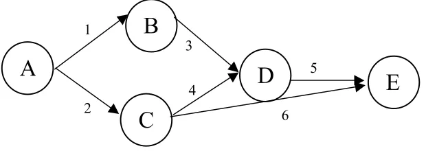
. Before proceeding, we illustrate thematerial by an example. Consider the network shown in Figure 1.
Clearly, (1,2) is a uniformly directed cut (UDC), because V is divided into two disjoint subsets X and
X
, where A∈
X and E∈
X
. The other UDCs of this network are (2,3), (1,4,6), (3,4, 6) and (5,6).Definition
3 Let D=E∪F be a uniformlydirected cut (UDC) of a network. Then, it is called an admissible 2-partition, if for any a∈F, we have
I
(
β
(
a
))
⊄
F
.To illustrate this definition, consider example 1, again. As mentioned before, (3,4,6) is a UDC. This cut can be divided into two subsets E and F. For example, E = {4}andF = {3,6}. In this case, this cut is an admissible 2-partition, because
I
(
β
(
3
))
= {3,4}⊄ F and alsoI
(
β
(
6
))
= {5,6}⊄F. However, if E = {6}and F = {3,4}, then the cut is not an admissible 2-partition, becauseI
(
β
(
3
))
= {3,4}⊂
F = {3,4}.For constructing the proper stochastic process, it is convenient to visualize the stochastic network as a PERT network, in which the arcs in the network represent the activities of a project. Duration of activity a∈A is assumed to be an exponentially distributed random variable with parameter
λ
a (the mean isa
λ
1
). Then, we try to find the distribution function of project completion time in the related PERT network.Definition
4 During the project execution and attime t, each activity can be in one of the active, dormant or idle states, which are defined as
A
B
D
E
C
1
2
4 3
6 5
follows:
i. Active: an activity is active at time t, if it is being executed at time t.
ii. Dormant: an activity is dormant at time t, if it is finished but there is at least one unfinished activity in
I
(
β
(
a
))
.If an activity is dormant at time t, then its successor activities inO
(
β
(
a
))
cannot begin.iii. Idle: an activity is idle at time t, if it is neither active nor dormant at time t.
The set of active and dormant states are denoted by Y(t) , Z(t), respectively and X(t)=(Y(t),Z(t)).
Consider example 1, again. If activity 3 is dormant, it means that this activity is finished but the next activity, i.e. 5, cannot start, because activity 4 is still active and not finished.
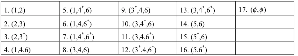
Table 1 presents all admissible 2-partition UDCs of this network. We use a superscript star to denote a dormant activity. All others are active. E contains all active, while F includes all dormant activities.
Now, let S denote the set of all admissible 2 - p a r t i t i o n U D C s o f t h e n e t w o r k , a n d
)}.
,
{(
φ
φ
∪
=
S
S
Note that X(t)=(
φ
,
φ
)
implies that Y(t)=φ
and Z(t)=φ
, i.e., all activities are idle at time t and hence the project is completed by time t. It can be proved that {X(t),t≥
0} is a continuous-time Markov process with state spaceS
, see Kulkarni and Adlakha [10] for the details of proof.As mentioned before, E and F contain active and dormant activities of a UCD,
respectively. When activity a finishes (with the rate of
λ
a), and there is at least one unfinished activity inI
(
β
(
a
))
, it moves from E to new dormant arcs set, i.e. to F'. Furthermore, if by finishing this activity its succeeding ones,O
(
β
(
a
))
, become active, then this set will also be included in the new E', whileI
(
β
(
a
))
will be deleted from E. Thus, the elements of the infinitesimal generator matrix of this process, denoted byQ
=
[
q
{(
E
,
F
),
(
E
,'
F
'
)}]
, where (E,F) and)
'
,'
(
E
F
∈
S
, are calculated as follow: In example 1, if E = {1, 2}, F =(
φ
)
and E' = {2,3}, F' =(
φ
)
, then E'=(E−{1})∪O(β(1)), and thus from Equation 5, q{(E,F),(E,'F')}=λ1. {X(t), t≥
0} is a finite-state absorbing continuous-time Markov process and since,
0
)}
,
(
),
,
{(
φ
φ
φ
φ
=
q
it can be concluded that this state is the absorbing one and obviously, the other states are transient. Furthermore, we number the states inS
such this Q matrix be an upper triangular one. We assume q [ (E,F) , E’,F’) ={ }
{ }
{ }
{ }
∪
=
′
−
=
′
−
=
′
⊄
∈
a
F
F
,
a
E
E
,
a
E
E
a
F
))
a
(
(
I
,
E
a
if
s
U
β
λ
(4){ }
{ }
−
=
∪
−
=
′
⊄
∈
))
(
(
I
F
'
F
))
(
(
)
a
E
(
E
a
F
))
a
(
(
I
,
E
a
if
a
α
β
α
β
β
λ
0
U
(5) TABLE 1. All Admissible 2-Partition Cuts of the Example Network.
1. (1,2)
5. (1,4
*,6) 9.
(3
*,4,6) 13.
(3,4
*,6
*)
17. )
(
φ
,
φ
2. (2,3)
6. (1,4,6
*) 10.
(3,4
*,6) 14.
(5,6)
3. (2,3
*) 7.
(1,4
*,6
*) 11.
(3,4,6
*) 15.
(5
*,6)
F
F
,
E
E
if
E
a a
′
=
′
=
∑
∈λ
(6)0 otherwise.
(7)States are numbered 1, 2, …, N =
S
. State 1 is the initial state, namely(
O
(
s
),
φ
);
and state N is the absorbing state, namely(
φ
,
φ
)
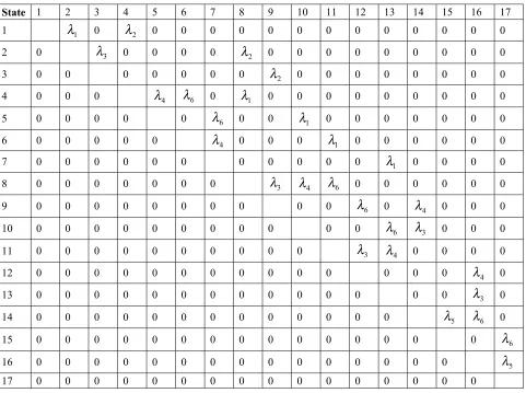
.Table 2 shows the infinitesimal generator matrix. The diagonal elements of the matrix Q are easily computed from (6). For example,
)
(
}
1
,
1
{
)}
2
,
1
(
),
2
,
1
{(
=
q
=
−
λ +
1λ
2q
.Let T represent the length of the longest path in the network. It is clear that T = min {t>0: X(t) = N/X(0) = 1}. Thus T is the time until {X(t), t
≥
0}gets absorbed in the final state starting from state 1.
Chapman-Kolmogorov backward or forward equations is applied to compute F(t) = P{T
≤
t} or the distribution function of longest path in the stochastic network . Using the backward algorithm, we define:Pi(t) = P{X(t) = N/X(0) = i} i = 1, 2, …, N (8)
Therefore, F(t) = P1(t). The system of differential equations for the vector P (t) = [P1 (t), P2 (t), …, PN(t)]T is given by:
P'(t) = Q.P(t)
(9) P(0) = [0,0,…,1]T
TABLE 2. Matrix Q Corresponding to the Example Network.
State 1 2 3 4 5 6 7 8 9 10 11 12 13 14 15 16 17
1
λ
1 0λ
2 0 0 0 0 0 0 0 0 0 0 0 0 02 0
λ
3 0 0 0 0λ
2 0 0 0 0 0 0 0 0 03 0 0 0 0 0 0 0
λ
2 0 0 0 0 0 0 0 04 0 0 0
λ
4λ
6 0λ
1 0 0 0 0 0 0 0 0 05 0 0 0 0 0
λ
6 0 0λ
1 0 0 0 0 0 0 06 0 0 0 0 0
λ
4 0 0 0λ
1 0 0 0 0 0 07 0 0 0 0 0 0 0 0 0 0 0
λ
1 0 0 0 08 0 0 0 0 0 0 0
λ
3λ
4λ
6 0 0 0 0 0 09 0 0 0 0 0 0 0 0 0 0
λ
6 0λ
4 0 0 010 0 0 0 0 0 0 0 0 0 0 0
λ
6λ
3 0 0 011 0 0 0 0 0 0 0 0 0 0
λ
3λ
4 0 0 0 012 0 0 0 0 0 0 0 0 0 0 0 0 0 0
λ
4 013 0 0 0 0 0 0 0 0 0 0 0 0 0 0
λ
3 014 0 0 0 0 0 0 0 0 0 0 0 0 0
λ
5λ
6 015 0 0 0 0 0 0 0 0 0 0 0 0 0 0 0
λ
616 0 0 0 0 0 0 0 0 0 0 0 0 0 0 0
λ
5where P(t) represents the system state vector and Q is the infinitesimal generator matrix of the stochastic process {X(t),t
≥
0}. By taking advantage of the upper triangular nature of Q, the differential Equations 9 can be easily solved.Therefore, if the waiting time in system for each queuing system is an exponential random variable, after transforming the queuing systems to the related stochastic arcs, we can use the above results to obtain the distribution function of longest path in the network of queues.
3.1. Networks of Queues with
M/M/
∞
Queuing Systems
The simplest case todetermine the longest path is a network, which includes only M/M/
∞
queuing systems. In this case, since no queue exists, the waiting time in the system is equal to the service time with exponential distribution. Therefore, each node having a queuing system is transformed into an exponential arc with parameterµ
, whereµ
is the service rate. After solving the system of differential Equations 9, the distribution function of longest path in the network is obtained.3.2. Networks of Queues with
M/M/1
Queuing Systems
In this case, the waitingtime density function in each M/M/1 queuing system is:
t
e
t
w
(
)
=
(
µ
−
λ
)
−(µ−λ) t>0 (10)where
λ
andµ
are the arrival rate and the service rate of this queuing system, respectively. Consequently, the system waiting time distribution is exponential with parameter (µ
-λ
). Therefore, we can transform each node into an exponential arc with parameter (µ
-λ
), and one can find the distribution function of longest path in the network, according to the proposed method.4. NETWORKS OF QUEUES WITH NON-MARKOVIAN QUEUEING SYSTEMS
Assume that the length of arc a∈A originating from the source node is a random variable with
density function f(t) and distribution function F(t). If N(t) represents the number of passages from this arc until time t, it is a non-homogeneous Poisson process with the following intensity function.
))
(
1
(
)
(
)
(
t
f
t
F
t
a
=
−
λ
(11)In this case, the probability of passage from this arc in the interval [t, t+
∆
t] is equal toλ
a(t)∆
t; given there has been no passage before t. It is clear thatλ
a(t) can be considered as a failure rate function; see Ross [15] for more details. Therefore, if the length of each arc a∈A, originating from the source node, is a random variable with general distribution function and the failure rate functiona
λ
(t), we should replaceλ
a in (4), (5) and (6) withλ
a(t). In this case, some elements of the first row of the infinitesimal generator matrix will be the functions of t. Thus, the system of linear differential equations with non-constant coefficients (12) has to be solved.P'(t)=Q(t).P(t)
(12) P(0)=[0,0,…,1]T
One should notice that the above equations can be applied only for the arcs originating from the source node, or if there is an M/G/
∞
queuing system in the source node. When another arc of the transformed stochastic network has the general distribution, the intensity function is a function of the starting time of traversing this arc, which is different from the quantity t in the differential Equations 12.The first differential equation of the system P'(t) = Q(t).P(t) corresponding to P1(t) has non-constant coefficients. Owning to the upper triangular nature of Q(t), we can easily solve the differential Equations 12. Let Q represent an (N-1)
×
(N-1) submatrix of Q(t) with the elimination of the first row and the first column of Q(t).where
T
N
t
P
t
P
t
P
t
P
(
)
=
[
2(
),
3(
),...,
(
)]
'
P (t)= Q .
P
(
t
)
)
0
(
P
=[0,0,…,1]T (13)Let M be the modal matrix of Q . That is, M is the (N-1)
×
(N-1) matrix whose N-1 columns are the eigenvectors of Q . Let)
N
(
...,
),
(
),
(
1
λ
2
λ
−
1
λ
be the eigenvaluesof Q , which are the diagonal elements of Q owning to the upper triangular nature of Q . We can compute
P
(
t
)
from Equation 14.)
(
t
P
=Me
ΛtM
−1P
(
0
)
(14)where
e
Λt is the diagonal matrix with ith diagonal element1
+
λ
(
i
)
t
+
...
(see Luenberger [11] for the details), thus:
=
− Λ
t N t
t
t
e
e
e
e
) 1 ( )
2 ( ) 1 (
.
.
0
.
.
.
.
.
.
0
0
.
0
λ λ
λ
Let q11(t) represent the element in the first row and first column of the matrix Q(t), and Q1(t) represent the N-1 row vector corresponding to the first row of Q(t) after the elimination of its first element, i.e. Q1(t)=
[
q
12(
t
),
q
13(
t
),...,
q
1N(
t
)
]
. Now, we should solve the following linear differential equation with non-constant coefficients.P'1(t)=q11(t).P1(t)+ Q1(t).
P
(
t
)
P1(0)=0Then P1(t) is computed from the following equation.
+
=
t
∫
s
Q
s
P
s
ds
C
t
P
1(
)
1
µ
(
)
tµ
(
)
1(
).
(
)
where
=
−∫
t
ds s q
e
t
11( ))
(
µ
. Taking into account the initial condition, the distribution function of longest pathis computed as follows:
=
t
∫
s
Q
s
P
s
ds
t
F
(
)
1
(
)
t(
)
1(
).
(
)
0
µ
µ
4.1. Networks of Queues with
M/G/
∞
Queuing System in the Source Node
Because of the limitations explained above, only the source node can contain an M/G/
∞
queuing system. If the source node contains an M/G/∞
queuing system, it can be transformed into an arc whose length is equal to the service time and its intensity function, orλ
(t), is equal to the failure rate function of the service time at time t. Then, the distribution function of longest path of the network is determined according to the method explained in section 4.Although in this case, the density function of the service time is not exponential, the steady-state density function of the time between two successive departures from the queuing system is exponential. Therefore, the departure process from this queuing system is a Poisson process, in which the departure rate would be equal to the arrival rate to the queuing system. See Gross and Harris [8] for more details.
4.2. Networks of Queues with
M/E
k/1
Queuing Systems
For this system, computingthe density function of the waiting time is not easy, compared with the previous ones. Therefore, for analyzing each M/Ek/1 queuing system with (
µ
, k) as the parameters of the Erlang distribution of service time, we consider only the special case that this queuing system must satisfy the heavy traffic assumption, which means its utilization factor should be approximately equal to 1.Theorem 1
. Considering the diffusionk+1 exponential series of arcs with parameters
2
)
2
(
σ
γ
−
,µ
,… ,µ
, whereγ
andσ
2 representthe expected value and the variance of the waiting time in queue.
Proof
. Assuming the heavy traffic assumption,the expected value and the variance of the waiting time in queue in each M/G/1 queuing system are:
)
t
(
O
t
)
)
S
(
E
(
t
=
−
∆
+
∆
∆
λ
1
γ
)
t
(
O
t
)
S
(
E
t
=
∆
+
∆
∆
22
λ
σ
where S represents the service time, and λ represents the arrival rate.
Let wq(x,t/x0) represent the density function of the waiting time in queue at time t, given that the waiting time in queue at time zero is equal to x0. It is proved that wq(x,t/x0) can be obtained from the Fokker-Planck equation, as follows:
∂wq(x,t/x0)/∂t=
-γ∂wq (x,t/x0)/∂x+σ2/2∂2wq(x,t/x0)/∂x2, with the following boundary conditions:
∫
0∞ wq(x,t/x0)dx=λ/γwq(x,t/x0)
≥
0In steady-state, the limiting density function exists, i.e. wq(x)=lim wq(x,t/x0), and can be computed as t→∞
follows:
σ2 / 2d2 w
q(x) / dx2 - γ dwq (x)/dx = 0
This is a second order differential equation with constant coefficients. Taking into account the following limiting boundary conditions under the heavy traffic,
∫
0∞ wq(x) dx = λ/γ≅
1wq(x)
≥
0It is concluded that:
wq(x) = (-2γ) / σ2 exp [(2γ) / σ2 x] x > 0
Therefore, the steady-state density function of the waiting time in queue is approximated by exponential with parameter (-2γ)/σ2.
We can decompose each random variable with Erlang distribution to a collection of structured random variables with exponential distributions; see Gross and Harris [8] for more details. The waiting time in queue has exponential distribution with parameter (-2γ)/σ2 and the service time can be decomposed to k exponential series arcs with parameter
µ
, and Theorem 1 is proved.Finally, we can find the distribution function of longest path in the network, according to the proposed method.
It should be noticed that the following theorem is also a new proof for this matter that the density function of the waiting time in queue in each M/G/1 queuing system in the steady state, taking into account the heavy traffic assumption, is exponential.
4.3. Networks of Queues with
G/M/1
Queuing Systems
If the arrival process toeach queuing system is the Poisson process, we have no G/M/1 queuing system in the network and we can easily find the rate of arrival process to each queuing system. In this case, if rij represents the probability that the customer whose service was finished in the service station settled in node i, goes to the service station settled in node j (rij, for all i and j
∈
V, are independent from the state of the system),i
λ
or the rate of arrival Poisson process to the service station settled in node i is given by:∑
∈=
V
j ji j
i
r
λ
λ
i∈
Vthis assumption that the arrival process to this node is the Poisson process with rate λ, the departure process from node u and also the arrival process to each node v
∈
V would not be the Poisson processes. However, we can compute the distribution function of time between two successive departures from node u by Equation 15. Let C (t) represent this distribution function and B(t) represent the distribution function of service time and ρ represent the utilization factor of this M/G/1 queuing system. C (t) is given by:C(t) = ρB(t) + (1-ρ)
∫
t0 B(t-u) λe
-λu du (15)
We can compute λu(t) or the rate of departure process from node u, which is equal to the failure rate function of the time between two successive departures from node u, from the following equation.
λu (t)=C'(t)/(1-C(t))
It is assumed that the departure process from node u has the independent increment. This assumption is reasonable, because the network is acyclic. Therefore, the departure process from node u can be considered as a non-homogeneous Poisson process with the intensity function λu(t).
Now, let N1(t) represent the arrival process from node u to node v and N(t) represent the departure process from node u. As mentioned, N(t) is a non-homogeneous Poisson process with the following distribution.
P[N(t)=m]=
(
)
!
0
0 ) (
0
≥
∫
∫
−
m
m
ds
s
e
sds t u mt u
λ
λ
Then, the rate of arrival process to node v from node u is proved to be equal to ruv λ u(t).
Theorem
2. N1(t) is a non-homogeneous Poissonprocess with the intensity function equal to ruvλu(t) or its distribution is
P[N1(t)=n]=
0
!
)
(
0 ) (
0
≥
∫
∫
−
n
n
ds
s
r
e
r sds t uv u nt u uv
λ
λ
Proof
.P[N1(t)=n]=
∑
∞
=n m
P[N1(t)=n/N(t)=m].P[N(t)=m]
P[N1(t)=n/N(t)=m]=
n
m
nuv
r
(1- ruv)m-nP[N1(t)=n] =
∑
∞
=n
m
n
m
nuv
r
(1- ruv)m-n
(
)
!
0 ) (
0
s
ds
m
e
s ds t u mt u
∫
∫
−λ
λ
P[N1(t)=n] =
A
B
D
C
E
k
m
p
n
l
n uv
r
(
)
!
0 ) (
0
s
ds
n
e
s ds t u nt u
∫
∫
−
λ
λ
∑
∞ =n m(1- ruv)m-n
(
)
(
)
!
0
s
ds
m
n
n m t
u
−
∫
λ
−P[N1(t)=n] =
n uv
r
(
)
!
0 ) (
0
s
ds
n
e
s ds t u nt u
∫
∫
−
λ
λ
. −
∫
t u uv sds
r
e
(1 )0λ( )P[N1(t)=n] =
0
!
)
(
0 ) (
0
≥
∫
∫
−
n
n
ds
s
r
e
r sds t uv u nt u uv
λ
λ
Corollary 1
. The rate of arrival process at eachnode k
∈
V isλ k(t)=
∑
∈V j
rjk λ j(t) k
∈
VProof
. The time between two successive arrivalsto node k is the minimum of some random variables, in which each one corresponds with the time between two successive arrivals from the node j
∈
V to node k. The failure rate function of this random variable is rjk λj(t), because the arrival process from node j to node k is a non-homogeneous Poisson process with the intensity function rjk λj(t), Therefore, the failure rate function of the minimum of these random variables, which indicates the rate of arrivalprocess to node k, would be equal to
∑
∈V jrjk λj(t).
In each node k
∈
V which contains an G/M/1 queuing system, if we obtain λk(t) or the rate of arrival process to this node, we can compute A(t) or the distribution function of time between two successive arrivals to node k from the following equation.A(t)=1- −
∫
t k udu
e
0λ ( )Assuming µ as the service rate of the G/M/1 queuing system, we can compute 0<x0 <1, or the unique root of Equation 16, by using a numerical method like the Newton-Raphson method.
Z=
∫
∞ − −0
) 1 ( z t
e
µ dA(t) 0<z<1 (16)After computing x0, we can compute the density function of the waiting time in system in the G/M/1 queuing system in this manner:
t x
e
x
t
w
(1 )0
)
01
(
)
(
=
µ
−
−µ − t>0It is clear that w(t) has exponential distribution with the parameter µ(1-x0), and we can transform this node to an exponential arc with the parameter
µ (1-x0).
TABLE 3. Characteristics of the Queuing Systems.
Node
Distribution of service
time
Number of servers
Parameters of the
distribution
A
Weibull
∞
(
α
,
β
)=(1,2)
B
Erlang
1
(
µ
,k)=(1,2)
C
Exponential
1
µ
C=4
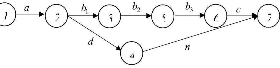
5. ILLUSTRATIVE EXAMPLE
Consider the network of queues depicted in Figure 2. Table 3 shows the characteristics of the service stations. There is no queuing system in node E. The other assumptions are as follows:
1. There is only one external arrival process to node A according to a Poisson process with the average of λ=0.98 per hour.
2. The arc lengths k, l, m, p are 0, but the length of arc n has exponential distribution with parameter 3.
3. Each customer after being served in node A goes to the service stations B or D with the equal probabilities (rAB=rAD=0.5).
According to the assumption 3, the arrival rate at the M/E2/1 queuing system settled in node B is equal to 0.5*0.98=0.49, and the utilization factor
of this queuing system is
ρB=2(0.49)=0.98
Therefore, the heavy traffic assumption is satisfied, and we can apply the diffusion approximation and the results of Theorem 1. The distribution function of time between two successive departures from node B, or C(t), is approximately equal to B(t), i.e., the distribution function of service time in this M/E2/1 queuing system, because ρB approaches 1. Since node C is connected to node B only through arc m, then C(t) is equal to A(t), i.e., the distribution function of time between two successive arrivals to node C. Therefore we conclude
A(t) = C(t) and C(t)
≅
B(t)⇒
A(t)≅
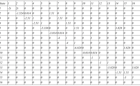
B(t) Now, we can compute x0, or the unique root of TABLE 4. Matrix Q(t) Corresponding to the Illustrative Example.z =
∫
∞0 e
-4t(1-z) te-t dt 0 < z <1
x0 = 0.043
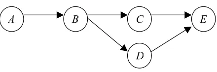
Now, each node containing a queuing system is transformed into an arc whose length is equal to the waiting time in system for this queuing system. Therefore, the network of queues is transformed to a stochastic network. Figure 3 shows this stochastic network.
Taking into account Figure 3, the M/G/
∞
queuing system settled in node A whose distribution of service time is Weibull with the density functionf
(
t
)
=
2
te
−t2 is replaced by arc a with the density functionλ
a(t)=2t, which is equal to the failure rate function of the service time. The waiting time in system in node B, which contains an M/E2/1 queuing system, is the sum of the waiting time in queue or b1 and the service time. Taking into account the heavy traffic assumption, the distribution of the waiting time in queue is exponential with the parameter1
b
λ
, which is computed as follows:γ=0.5 λE(S)-1=-0.02
σ2 = 0.5 λE (S2) = 0.49 (Var (S) + (E (S) )2) = 0.49 (2+4) = 2.94
1
b
λ
= (-2γ)/σ2 = 0.014According to the Theorem 1, the service time is replaced by two series arcs b2 and b3, in which both of them have exponential distributions with parameter 1. Arc c indicates the waiting time in system in G/M/1 queuing system settled in node C, which has exponential distribution with this parameter:
λ
c=µC (1-x0)=4(1-0.043)=3.828Arc d indicates the waiting time in system in M/M/1 queuing system of node D, which has exponential distribution with this parameter:
d
λ
= (µD - 0.5λ) = 2 - 0.49 = 1.51Arc n indicates the length of arc n in the original network, which has exponential distribution with parameter
λ
n=3.Now, we want to find the distribution function
1
3
4
7
2
5
6
a
b
1d
n
c
2
b
b
3Figure 3. The stochastic network corresponding to the illustrative example.
A
B
C
D
of longest path from node 1 to node 7 in the stochastic network, which is equal to the distribution function of longest path from node A to node E in the original network of queues. The indicated stochastic process {X(t),t
≥
0} has 16 states in this order:)}
,
(
),
n
*,
c
(
),
d
*,
c
(
*),
n
,
c
(
*),
n
,
b
(
*),
n
,
b
(
*),
n
,
b
(
),
n
,
c
(
),
n
,
b
(
),
n
,
b
(
),
n
,
b
(
),
d
,
c
(
),
d
,
b
(
),
d
,
b
(
),
d
,
b
(
),
a
{(
S
φ
φ
3 2 1 3 2 1 3 2 1=
Therefore, the infinitesimal generator matrix Q(t) has 16 states. Table 4 shows the infinitesimal generator matrix Q(t). The arc parameters are as follows:
a
λ
(t) = 2t,1
b
λ
= 0.014,2
b
λ
= 1,3
b
λ
= 1,c
λ
= 3.828,λ
d = 1.51,λ
n =3Then, we solve the following system of differential equations with non-constant coefficients.
P'16(t) = 0
P'15(t) = -3P15(t)+3P16(t)
P'14(t) = -1.51P14(t)+1.51P15(t)
P'13(t) = -3.828P13(t)+3.828P16(t)
P'12(t) = -P12(t)+P13(t)
P'11(t) = -P11(t)+P12(t)
P'10(t) = -0.014P10(t)+0.014P11(t)
P'9(t) = -6.828P9(t)+3P13(t)+3.828P15(t)
P'8(t) = -4P8(t)+P9(t)+3P12(t)
P'7(t) = -4P7(t)+P8(t)+3P11(t)
P'6(t) = -3.014P6(t)+0.014P7(t)+3P10(t)
P'5(t) = -5.338P5(t)+1.51P9(t)+3.828P14(t)
P'4(t) = -2.51P4(t)+P5(t)+1.51P8(t)
P'3(t)=-2.51P3(t)+P4(t)+1.51P7(t)
P'2(t)=-1.524P2(t)+0.014P3(t)+1.51P6(t)
P'1(t)=-2tP1(t)+2tP2(t)
Pi(0)=0 for i=1,2,…,15 P16(0)=1
According to the proposed method in section 4, we initially compute
P
(
t
)
from Equation 14. Then we obtain Q1(t).P
(
t
)
in this manner:t . t . t . t t t . t . t t . t t . t . t t .
e
t
.
e
t
.
e
t
.
e
t
.
e
t
.
e
t
.
e
t
.
e
t
.
e
t
.
e
t
.
e
t
e
t
.
e
t
.
e
t
.
t
)
t
(
P
t
)
t
(
P
).
t
(
Q
524 1 014 3 014 0 4 2 2 51 2 51 2 2 4 338 5 51 1 828 6 3 828 3 2 1294
4
112
2
016
2
038
0
038
0
128
0
076
0
064
0
002
0
132
0
4
001
0
028
2
002
0
2
2
− − − − − − − − − − − − − −+
−
−
+
+
−
−
+
−
−
−
+
+
+
=
=
Finally, F(t)=P1(t) is obtained in this manner:
∫ − − − − − − − − − − − − − − − + − − + + − − + − − − + + + = t s s s s s s s s s s s s s s s s s s s s s s s s s s s s s t ds se se se e s e s se e s se se se se se se se se e t F 0 524 . 1 014 . 3 014 . 0 4 2 2 51 . 2 51 . 2 2 4 338 . 5 51 . 1 828 . 6 3 828 . 3 2 2 2 2 2 2 2 2 2 2 2 2 2 2 2 2 294 . 4 112 . 2 016 . 2 038 . 0 038 . 0 128 . 0 076 . 0 064 . 0 002 . 0 132 . 0 4 001 . 0 028 . 2 002 . 0 2 ) (
We can easily compute the moments of the distribution, using a suitable numerical integration technique. We used MATLAB 5.3 to compute the expected value and the variance of the longest path in the indicated network of queues. Theses values are as follows:
µ=
∫
∞2 0
2
2
(
)
µ
σ
=
∫
∞t
dF
t
−
=5020.6166. COMPUTATIONAL EXPERIENCE
For showing the validity of the proposed method, we solve 4 new numerical examples. All of these networks have 4 service stations, but with different configurations and characteristics of the service stations. The arc lengths are all assumed to be equal 0.
Case I is depicted in Figure 4. This is a serial network of queues. The arrival process to the source node of this network is assumed to be a Poisson process with the rate of λ=1 per hour. Node A contains an M/G/
∞
queuing system with the Weibull distribution of service time and the parameters (α,β) = (1,2). Nodes B and D contain the M/M/1 queuing systems with the service rates equal to µB=µD=2. Node C contains an M/M/∞
queuing system with the service rate equal toµC=1. Figure 5 shows the transformed stochastic network.
In this case, the size of the state space is equal
to 5,
S
=
{(
1
),
(
2
),
(
3
),
(
4
),
(
φ
,
φ
)}
, and F(t) is given by∫
− − −−
−
−
−
=
e
t tse
ss
e
s ss
e
s sse
s sds
t
F
0
2
3 2 2 2
2 2
2
2
2
)
(
Case II is depicted in Figure 6. The configuration of this network is the same as the illustrative example, except that there is no non-Markovian queuing system in the nodes of this new network. The arrival process is a Poisson process with the rate of λ=2 per hour. Node A contains an M/M/
∞
queuing system with the service rate equal to µA=3. Nodes B, C and D contain the M/M/1 queuing systems with the service rates equal to µB=2, µC=4 and µD=2, respectively. There is no queuing system in node E. It is also assumed that rAB = rAD = 0.5. Figure 7 shows the transformed stochastic network.In this case, the size of the state space is equal to 7,
)}
,
(
),
4
,
3
(
),
4
,
3
(
),
4
,
3
(
),
4
,
2
(
),
4
,
2
(
),
1
{(
* * *φ
φ
=
S
and F (t) is given by
t t
t t
t
e e
e te
e t
F
3 2
4 3
25 . 3 5
. 4
5 . 1 5
. 1 75 . 3 1 ) (
− −
− −
−
− +
+ +
− =
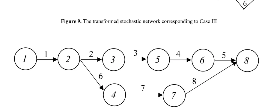
Case III is depicted in Figure 8. This is the first network of queues that we analyze and has more than one G/M/1 queuing system. The arrival process is a Poisson process with the rate of
λ=0.49 per hour. Node A contains an M/G/
∞
queuing system with the Weibull distribution of service time and the parameters (α,β)=(2,2). Node B contains an M/E2/1 queuing system with1
1
2
2
3
3
4
4
5
Figure 5. The transformed stochastic network corresponding to Case
A
B C
D E
the service parameters equal to (
µ
, k)=(1,2). Nodes C and D contain the G/M/1 queuing systems with the service rates equal to µC=4 andµD=2, respectively. There is no queuing system in node E. It is also assumed that rBC = 0.8 and rBD = 0.2. Figure 9 shows the transformed stochastic network.
In this case, the size of the state space is equal to 8,
)}
,
(
),
6
,
5
(
),
6
,
5
(
),
6
,
5
(
),
4
(
),
3
(
),
2
(
),
1
{(
* *φ
φ
=
S
,and F(t) is given by:
∫
− − − − − − −−
+
+
−
+
+
=
t s . s s s s s s . s s . s s . s s tds
e
s
.
e
s
.
e
s
.
e
s
.
e
s
.
e
s
.
se
e
)
t
(
F
0 014 0 2 2 2 2 841 5 2 956 1 2 885 3 2 2 2 2 2 2 2 2 2 2 2152
4
12
0
124
0
0004
0
032
0
002
0
4
The configuration of the network of queues in Case IV is the same as the illustrative example, Figure 2, except that node D contains an M/E2/1 queuing system with the service parameters equal to (
µ
,k)=(1,2) instead of the M/M/1 queuing system, and the arc lengths of this new network are all equal to 0. This is the first network of queues that we analyze and has more than one M/Ek/1 queuing system. Figure 10 shows the transformed stochastic network.In this case, the size of the state space is equal to 19
)}.
,
(
),
,
(
),
,
(
),
,
(
),
,
(
),
,
(
),
,
(
),
,
(
),
,
(
),
,
(
),
,
(
),
,
(
,
to
),
,
(
),
,
(
),
,
(
),
,
(
),
,
(
),
,
(
),
{(
S
* * * * *φ
φ
8
5
8
5
8
5
7
5
6
5
8
4
8
4
7
4
6
4
8
3
8
3
19
7
3
6
3
8
2
8
2
7
2
6
2
1
=
F(t)
is also given by:
∫
+ + + − − − + + + + − = − − − − − − − − − − − − t s s s s s s s . s s . s s . s s . s s s s . s s s s . s s t ds e s . e s . se . e s . se . se . se e s . se . se . se . se . e ) t ( F 0 2 3 2 2 2 014 1 2 842 3 014 1 028 0 2 828 3 014 0 2 2 2 2 2 2 2 2 2 2 2 2 2 0006 0 002 0 002 0 066 0 001 0 118 0 2 064 0 001 0 114 0 88 3 882 1By comparing these four cases and also the
illustrative example with each other, it is
concluded that the size of the state space is
dependent on the number of service stations,
the number of arcs, and also the number of
M/E
k/1
queuing systems settled in the nodes of
1
1
2
2
3
3
4
4
Figure 7. The transformed stochastic network corresponding to Case II.
A B C E
D
the network of queues. All of these
5
cases
have the equal number of service stations, but
Case IV, which has the maximum number of
arcs and
M/E
k/1
queuing systems between
these
5
cases, has the maximum size of the
state space equal to
19
, and consequently,
Case I has the minimum size of the state space
equal to
5
.
Therefore, the worst case of the problem
would be a complete network of queues with
maximum number of
M/E
k/1
queuing systems,
in which each node should contain a service
station.
7. CONCLUSION
In this paper, we developed an analytical method to determine the steady-state distribution function of longest path in networks of queues on the basis of stochastic process, queuing theory and also graph theory. Furthermore, we assumed the arc lengths are independent random variables. Several problems in the fields of project
management, production systems, reliability modeling and computer networks can be formulated as a network of queues and then apply this method.
In the proposed method, the network of queues is transformed into a stochastic network. Then, we obtain the distribution function of the steady-state longest path by solving a system of linear differential equations corresponding to the related continuous-time Markov process. If the service times and the arc lengths are exponential random variables, then the coefficients of the system of linear differential equations are constant and can be easily solved. However, if any of those random variables has the general distribution, the resulting system of linear differential equations has non-constant coefficients, and can be solved through the analytical method, which described in section 4.
The limitation of this model is that the state space can grow exponentially with the network size. As the worst-case example, for a complete transformed network with n nodes and
n
(
n
−
1
)
2
arcs, the size of the state space is given by1
1
2
2
3
3
4
4
5
5
6
6
Figure 9. The transformed stochastic network corresponding to Case III
1
3
4
6
7
8
2
5
1
2
3
4
5
8
7
6
1
)
(
n
=
U
n−
U
n−N
, where∑
=−
=
nk
k n k n
U
0 ) (
2
Refer to Kulkarni and Adlakha [10].
In practice, the number of arcs in PERT networks is generally much less than
n
(
n
−
1
)
2
, and it should also be noted that for large networks any alternate method of producing reasonably accurate answers will be prohibitively expensive. In this paper, we analyzed the acyclic networks with no direct or indirect feedback or overtaken. Therefore, it can be assumed that the waiting time in the queuing systems are independent random variables. Other limitation of this model is that the waiting time in the queuing systems settled in the nodes of the network are not always independent, and we have some limitations to use the independency assumption.This model can be extended to the networks
of queues, which contain the other kinds of
queuing systems.
8. REFERENCES
1. Ad lakh a, V . an d Ku lkarn i, V . A., “Classified Bibliography of Research on Stochastic PERT Networks: 1966-1987”, INFOR 27, (1989), 272- 290.
2. Azaron, A. and Fatemi Ghomi, S. M. T., “Optimal Control of Service Rates and Arrivals in Jackson Netwo rks”, Euro p ea n J o u rna l o f Op era t i o n a l Research, 147, (2003), 17-31.
3. Bo n d y, J. an d M u rty, U. , “Grap h Th eo ry wi t h Applications”, Elsevier Publishing Co., Inc., (1976). 4. Burt, J. and Garman, M., “Conditional Monte Carlo: A Simulation Technique for Stochastic Network Analysis”, Management Science, 18, (1971), 207-217.
5. Charnes, A., Cooper, W. and Thompson, G., “Critical Path Analysis via Chance Constrained and Stochastic Programming”, Operations Research, 12, (1964), 460-470.
6. Elmaghraby, S., “On the Expected Duration of PERT Type Networks”, Management Science, 13, (1967), 299-306.
7. Fishman, G., “Estimating Critical Path and Arc Probabilities in Stochastic Activity Networks”, Research Logistic Quarterly, 32, (1985), 249-261.
8. Gross, D. and Harris, M., Fundamentals of Queuing Theory, 2nd Edition, John Wiley and Sons, (1985). 9. Hopfinger, E. and Steinhardt, V., “On the Exact
Evaluation of Finite Activity Networks with Stochastic Durations of Activities, (Lecture Notes in Economics and Mathematical Systems, Vol. 117, Optimization and Operations Research), Springer-Verlag. (1976).
10. Kulkarni, V. and Adlakha, V., “Markov and Markov Regenerative PERT Networks, Operations Research, 34, (1986), 769-781.
11. Luenberger, D., “Introduction to Dynamic Systems”, John Wiley and Sons. (1979).
12. Martin, J., “Distribution of the Time Through a Directed Acyclic Network”, Operations Research, 13, (1965), 46-66.
13. Ord, J., “A Simple Approximation to the Completion Time Distribution for a PERT Network”, Journal of Operational Research Society, 42, (1991), 1011-1017.
14. Robillard, P., “Expected Completion Time in PERT Networks”, Operations Research, 24, (1976), 177-182.
15. Ross, S. “Stochastic Process”, 2nd Edition, John Wiley and Sons, (1996).
16. Soroush, H., “The Most Critical Path in a PERT Network”, Journal of Operational Research Society, 45, (1994), 287-300.