Assessing the temporal stability of spatial patterns of soil apparent electrical
conductivity using geophysical methods
Sunshine A. De Caires*, MarkN. Wuddivira, and Isaac Bekele
Department of Food Production, University of West Indies, St. Augustine, Trinidad and Tobago, West Indies
Received December 12, 2013; accepted July 14, 2014 Int. Agrophys., 2014, 28, 423-433
doi: 10.2478/intag-2014-0033
*Corresponding author e-mail: [email protected] A b s t r a c t. Cocoa remains in the same field for decades, resulting in plantations dominated with aging trees growing on variable and depleted soils. We determined the spatio-temporal variability of key soil properties in a (5.81 ha) field from the International Cocoa Genebank, Trinidad using geophysical methods. Multi-year (2008-2009) measurements of apparent elec-trical conductivity at 0-0.75 m (shallow) and 0.75-1.5 m (deep) were conducted. Apparent electrical conductivity at deep and shallow gave the strongest linear correlation with clay-silt content (R = 0.67 andR = 0.78, respectively) and soil solution electrical conductivity (R = 0.76 and R = 0.60, respectively). Spearman rank correlation coefficients ranged between 0.89-0.97 and 0.81-0.95 for apparent electrical conductivity at deep and shallow, respectively, signifying a strong linear dependence between meas-urement days. Thus, in the humid tropics, cocoa fields with thick organic litter layer and relatively dense understory cover, experi-ence minimal fluctuations in transient properties of soil water and temperature at the topsoil resulting in similarly stable apparent electrical conductivity at shallow and deep. Therefore, apparent electrical conductivity at shallow, which covers the depth where cocoa feeder roots concentrate, can be used as a fertility indicator and to develop soil zones for efficient application of inputs and management of cocoa fields.
K e y w o r d s: apparent electrical conductivity, electromag-netic-induction, humid tropics, spatial patterns, temporal stability
INTRODUCTION
Cocoa (Theobroma cacao L.) plantations have a
prob-lem of within-field yield variability which may originate
form spatial variation is soil properties (Eneje et al., 2012;
Obalum et al., 2013). Once established, cacao remains in
the same field for decades, therefore cocoa fields are domi
-nated with aging trees growing on variable and depleted
soils (Snoeck et al., 2010). In Trinidad and Tobago like
many cocoa producing countries, increase in cocoa pro-duction is mainly due to expansion of existing farms or creation of new farms rather than increase in yield per
unit area (Gockowski, 2007; Snoeck et al., 2010). While
technological approaches to address within-field
variabi-lity have resulted in stupendous increase in yield per unit area in the production of other crops, cocoa production still
relies on inefficient and outdated traditional production and
management methods that do not take into account
within-field soil variability. Uniform management of large cocoa
plantations have resulted in less than optimum yields and
economic returns due to nutrient deficiencies as well as
excessive fertilizer application that may potentially reduce
environmental quality (Schumann et al., 2003). Therefore,
there is an emerging need for cocoa producers to increase
input efficiency, improve the economic margins of crop
production, and reduce environmental risks, which can be
achieved if site-specific precision management of planta
-tions is employed.
Precision agriculture seeks to develop agronomic
stra-tegies to manage spatially variable fields more efficiently by developing management zones or subregions of a field
with homogeneous yield-limiting factors (Doerge, 1999;
Rossi et al., 2013). This holistic system approach depends
on understanding and accurately identifying the
underly-ing factors responsible for variation in crop yield (Mann et
al., 2011). Since soils and their properties play a distinctive
role in determining the productivity of agricultural fields,
once a sound understanding of the within-field
variabi-lity of soil physicochemical properties in cocoa plantations
is established, management zones can be developed and recommendations made for varying inputs. Apparent soil
electrical conductivity (ECa) has shown great potential for
identifying yield limiting soil properties and used
success-fully to develop management zones (Mann et al., 2011;
Moral et al., 2010).
Electromagnetic induction (EMI) sensors such as DUALEM-1S EC meter employ geophysical imaging tech-niques to rapidly, non-invasively measure spatial variations
of soil ECa (Atwell et al., 2013; Bréchet et al., 2012; Rossi
et al., 2013; Wuddivira et al., 2012). Apparent soil electri-cal conductivity correlates with va rious physicochemielectri-cal
soil properties such as salinity (Rhoades et al., 1999), clay
content (Triantafilis and Lesch, 2005; Wuddivira et al.,
2012), water content (Haimelin, 2008) and carbon content
(Martinez et al., 2009). Recently, Atwell et al. (2013) and
Bréchet et al. (2012) showed that under humid tropical
conditions, variation in ECa was influenced by temporal
changes in soil moisture content, spatial variation of clay-silt mineral content, soil solution electrical conductivity (ECe) and soil water repellency. Thus, EMI sensors pro-vide the prospect of cost effectively collecting dense spatial
data, combining sufficient scale triplet of spacing, extent
and support to capture small and large scale variability of
soil properties (Atwell et al., 2013).
Electromagnetic induction measurements using DUALEM-1S EC meter are sensitive to the upper 0-0.75 m
for ECas and the lower 0.75-1.5 m for ECad, making it
espe-cially beneficial to management zone development in cocoa
plantations, since cocoa trees obtain moisture and nutrients from a mat of lateral roots which lie in the top 0.2 m (Wood and Lass, 1985). Although, researchers have investigated the spatio-temporal stability of ECa in temperate regions
(King et al., 2001; Nehmdahl and Greve, 2001), there has
been limited research on tropical soils (Robinson et al.,
2009). Even so, there are no reports of studies on cocoa soils using geophysical imaging to assess the temporal stability of spatial patterns of ECa to develop management zones. Temporal stability is important in order to make mana- gerial agricultural decisions based on spatial variability. King
et al. (2001) and Nehmdahl and Greve (2001) both noted that in order to characterize ECa, multiple surveys yielding similar patterns over time, regardless of external factors, should be undertaken. This is of vital importance if zones developed based on ECa patterns are to be used to manage
the field for multiple years (Farahani and Buchleiter, 2004),
as would be the case for cocoa plantations.
Farahani and Buchleiter (2004) compared the stability
of ECas and ECad in three irrigated sandy fields in eastern
Colorado and found ECad to be more temporally stable than
the corresponding ECas. This was expected as the top soil
layer is subjected to more fluctuation in transient properties
such as water content (WC) and temperature. The magnitude
of fluctuation depends on climatic factors (rainfall and tem
-perature) and the type of crop cover. Fluctuations in the top
soil layer will therefore be more pronounced in semi-arid
regions and in fields cultivated to annual crops resulting in
more temporally unstable ECas than in the humid tropics in
fields grown to permanent tree crops. We hypothesize that
due to the perennial nature of cocoa trees, thick organic
lit-ter and understory cover coupled with little fluctuation in
soil water and temperature in the humid tropics, ECas will
be as temporally stable as ECad. The objectives of our study
were to:
-investigate the temporal stability of spatial patterns of apparent soil electrical conductivity,
-determine which soil properties contribute to
electromag-netic induction signals in a humid tropical cocoa field.
MATERIALS AND METHODS
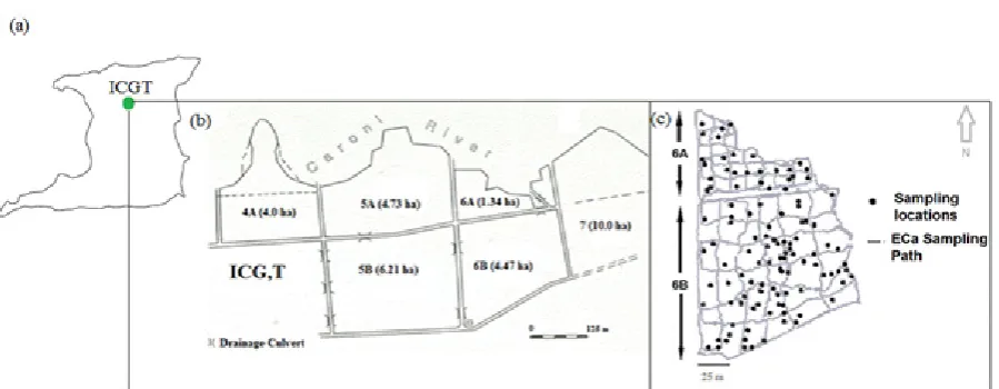
The study was conducted at the International Cocoa Genebank, Trinidad (ICG, T), 10° 34’ 39” N, 61° 18’ 0” W (Fig. 1a). The ICG, T consists of 33 ha of land divided into
five fields (Fig. 1b). Cocoa plants were established between
1986 and 1990. Permanent shade was provided by Erythina spp. and temporary shade by the original ‘old’ cocoa trees and non-commercial bananas (Musa acuminate). Our study
was conducted on a 5.81 ha field (blocks 6A and 6B) that is prone to seasonal flooding by the Caroni River, which
may redistribute soil particles, alter the absolute
magni-tude of ECa and flush any fertilizer salts from the soil that
may build up from previous growing seasons. The ICG, T is subjected to humid tropical conditions, with mean annual rainfall of 2000 mm falling mainly between July and December (wet season) and a marked dry season from January to June, with less than 400 mm of rain (Granger, 1983). Average monthly temperatures range from 25.7 to 28.9°C, with an average monthly relative humidity of 81%.
The ICG, T is sited on a fine silt-clay alluvium belonging to
the Cunupia clay soil series (Inceptisol), which has
restrict-ed internal drainage and a flat topology.
The DUALEM-1S EC meter (Dualem, Milton, ON,
Canada) described in Abdu et al. (2007) was used to carry
out ECa mappings. The sensor was connected to an Archer
Ultra Rugged-Pda field computer (Juniper Systems, Logan,
UT) running HGIS software (Starpal, Ft, Collins, CO) and a GPS (REB-12R, RoyalTek, Tao Yuan, Taiwan)
contain-ing a SirfIII chipset. The sensor-field computer-GPS setup
provided spatially exhaustive geo-referenced readings for
ECas and ECad. Using the time lapse approach (Robinson
et al., 2009), a total of nine ECa surveys were completed between 2009 and 2010. This was done to capture multi-year spatio-temporal and seasonal changes of ECa in the
cocoa field. The EMI instrument was held constantly at
ASSESSING THE TEMPORAL STABILITY OF SPATIAL PATTERNS USING GEOPHYSICS 425
The first EMI image was made on March 13, 2009 in the
middle of the dry season. The next two images were taken towards the end of the dry season on the April 28 and May 18, 2009. Wet season surveys were performed on June 30,
August 24, September 26 and November 27, 2009. The final
two images were obtained during the dry season in 2010 on January 21 and June 30. Soil water content, measured with a theta probe (DeltaT Devices, Burwell, Cambridge, United Kingdom) and soil temperature, measured with a soil tem-perature sensor (Novel Ways Ltd, Hamilton, New Zealand)
were recorded before and after the first three ECa surveys
(data not shown). The soil temperature did not change from
30oC, which is consistent for tropical climates (Robinson et
al., 2009). Therefore, no temperature correction was
need-ed for the data.
Data were downloaded from the field computer and
subjected to QA/QC analysis to recognize and exclude data points that where obtained while the surveyor was station-ary. Using a time-series view of the data, ECa values were then checked for stability and any erratic values were elim-inated. As a quality control measure, inconsistent values caused by materials such as buried metal fragments, wires
and pipes were identified and removed from the dataset.
The datasets were normal score transformed using S-GeMS (Remy, 2005) to prepare the data for a kriging process. The underlying assumption of kriging was that the data were normally distributed (Goovaerts, 2010). The nor-mal score transformation was useful in transforming data with large outlying values to provide a normal distribution with a mean of 0 and a variance of 1. The normal score trans-form function was derived by matching the original skewed cumulative distribution function (cdf) to a standard normal
cdf. Block kriging was performed on each dataset by fitting
them with variograms and kriging them on a 5 x 5 m grid
using VESPER (Walter et al., 2001). The final ECa maps
were created in S-GeMS, where the kriged data were back transformed.
Vachaud et al. (1985) used the differences between
individual and spatial average values and Spearman rank correlation to characterize the temporal stability of para-metric values. The method depends on a spatial location keeping its rank in the cdf for different sampling times
(Vachaud et al. 1985). Since the study site was topologically
flat, the supposition was that EMI mapping can capture the
dominant intrinsic physical soil property through repeated mapping, by employing a temporal stability analysis
tech-nique. Ranking and/or time-lapse ECaimages were used
successfully by Robinson et al. (2009) to identify
hydro-logic subsurface patterns, soil texture, and water-holding
capacity. The modified temporal and rank stability proce
-dure described by Robinson et al. (2009) was employed
in this study to determine the stability of ECas and ECad
across the field.
Prior to soil sample extraction at the depth of 30 cm from 120 random sampling sites using a Dutch Cutting Auger, EMI signal (ECa) and GPS coordinates were recorded for each sites. Soil samples were transported back to the lab in Ziploc plastic bags to prevent moisture loss. Sub-samples of approximately 105 g of soil (fresh weight) were taken from each sample and analysed for gravimetric water
con-tent (θg) by recording dry mass after oven-drying at 105º
C until constant weight was achieved. The rest of the soil was air dried, and stones and organic debris such as roots were removed from the samples. The samples were then crushed using a mortar and a pestle and passed through a 2 mm sieve. Particle size distribution, ECe and organic mat-ter content (OM) were analysed using standard methods.
pH measurements were made in 0.01 M CaCl2 (soil to
solu-tion ratio 1:1) using a pH meter equipped with combinasolu-tion
gel-filled glass electrode.
RESULTS AND DISCUSSION
Summary statistics of ECa are presented in Table 1.
Mean ECa values varied from 10.98 to 21.85 mS m-1 for
ECad and 3.77-17.29 mS m-1 for ECa
s. ECas data ranged
from 1.00 to 37.10 mS m-1 while ECa
d ranged from 0.63 to
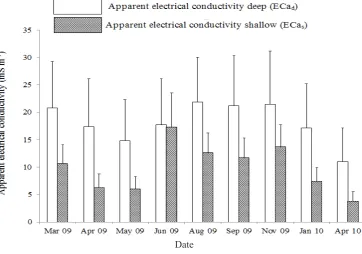
86.10 mS m-1. June 2009 exhibited very close mean ECa
s
and ECad values (Fig. 2), indicating that both depths had
similar water content and temperatures on that day. Spatial
variability, as quantified by coefficient of variation (CV),
was generally high for all mapping events, ranging from 28.91 to 55.87%. Farahani and Buchleiter (2004)
report-ed similar variation in CV in three irrigatreport-ed sandy fields
in eastern Colorado, seemingly a normal range for low salt systems. Both absolute and relative measures of va- riability such as standard deviations (Stdev, 1.73 to 9.77)
and CV (28.91% to 55.87%) for the nine ECas and ECad
surveys were generally high at all sites, indicating that
rainfall and temperature fluxes affected the variability of
ECa among survey dates. This interpretation is supported
by the Spearman rank correlation coefficient (rs) of ECa
measurements (Table 2), where correlations are high for the
wettest months surveyed. ECas had lower means, standard
deviations, and CVs than ECad indicating less variability,
which is not expected due to more exposure to climatic and
anthropogenic disturbances. Moderate (0.36 < |R2| < 0.64)
to strong (|R2| > 0 .64) positive coefficients of determina
-tion, R2 (Fig. 3) were observed between ECa
s and ECad for
all measurement days, suggesting homogeneity between
shallow and deep horizons, although this is partly due to deep ECa integrating the 1.5 m soil that includes the
0.75 msoil layer represented by ECas (Farahani and
Buchleiter, 2004).
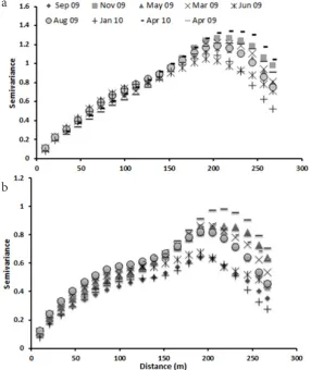
The normal score semivariograms in Fig. 4 demonstrate
strong spatial structure and correlation. ECad variograms
had a slightly different structure than the ECas models.
ECas models had slightly larger nugget, lower sill and ge-
nerally shorter range values (except for April and May 2009)
than corresponding ECad models (Table 3) suggesting ECas
is less spatially continuous than ECad. The least error in the
measured ECa was observed in the driest month of January
2010, which had the smallest nugget effect for both ECas
and ECad. Spherical semivariograms were fitted to both
ECas and ECad, because spherical models exhibit linear
behaviour at the origin and are appropriate for represent-ing properties with a higher level of short-range variability (Bohling, 2005). The different environmental conditions under which data was collected had only minor effects on the spatial structure of the ECa semivariograms
signify-ing that spatial dependence isn’t significantly affected by
ephemeral factors, although absolute values may change.
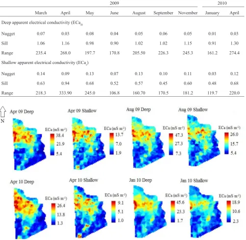
Kriged ECas and ECad maps for April 2009 and April
2010 (same month, consecutive years), August 2009 (wettest survey month) and January 2010 (driest survey month) are presented in Fig. 5. Visual inspection of all maps reveals a general pattern where a zone with higher ECa approximately 50 m x 100 m was observed. For all
T a b l e 1. Summary statistics of deep (ECad) and shallow (ECas) apparent soil electrical conductivity
Sampling
date ECad (mS m
-1) ECa
s (mS m-1)
Min Max Mean Std CV Min Max Mean Std CV
Dry season (2009)
March 4.50 48.62 20.84 8.43 40.43 3.10 23.50 10.66 3.44 32.30
April 1.26 86.10 17.40 8.70 49.99 1.80 13.60 6.26 2.46 39.28
May 0.65 42.34 14.84 7.46 50.27 1.69 16.70 6.02 2.25 37.35
Wet season (2009)
June 4.08 54.07 17.71 8.40 47.42 6.40 37.10 17.29 6.28 36.35
August 7.30 49.04 21.85 8.20 37.53 5.40 26.00 12.59 3.64 28.91
September 2.13 53.26 21.23 9.15 43.09 4.80 31.80 11.68 3.66 31.34
November 0.63 57.82 21.43 9.77 45.58 6.60 34.80 13.70 4.04 29.51
Dry season (2010)
January 1.74 44.95 17.12 8.09 47.22 2.30 18.90 7.36 2.61 35.44
ASSESSING THE TEMPORAL STABILITY OF SPATIAL PATTERNS USING GEOPHYSICS 427
ECas, R = 0.23) and θg (ECad, R = 0.28; ECas, R = 0.25)
were weak at both depths, they were found to be significant at the 5% level (Table 5). Coefficient of variability (CV)
for soil propertiesindicated significant spatial variability,
suggesting the convenienceof defining management zones
(Moral et al., 2010).
Given the varying texture and ECe across the field
as indicated by the CVs, clay-silt content and ECe were expected to give the strongest correlations with the ECa signal. Although ECa is known to be strongly dependent on water content, the sampling on a single day, at a point in time, does not capture the temporal change in water content given different texture-dependent calibrations (Robinson
et al., 2009). Stepwise multiple regressions indicated that
the most important predictors of ECad were ECe, clay-silt
content and OM, in that order, whereas the most important
predictors of ECas were clay-silt content, then ECefollowed
by θg. The regression model suggested that ECe and
clay-silt content dominated the ECad signal response accounting
for 67% of its variability, whereas clay-silt content alone
explained 61% of the ECas signal response. Due to more
exposure to climatic and anthropogenic disturbances,
including frequent flooding, ECas response was dominated
by varying soil particle size distributions across the field.
Concomitantly, the ECad signal was most influenced by
ECe suggesting that salts accumulate as soil depth increas-es. The ICG,T’s restricted internal drainage indicates clay content increase as soil depth increases, which explains the increase in salt accumulation with depth.
maps, the south-western end of the field had the lowest ECa
values and the north-eastern side had the highest. Maps of April 2009 and April 2010 showed a lot of variability, espe-cially at the deeper depths. Both surveys were done during a rainfall event and the pattern was interpreted to indicate the redistribution of water, changing the soil ECa as the
field was mapped.
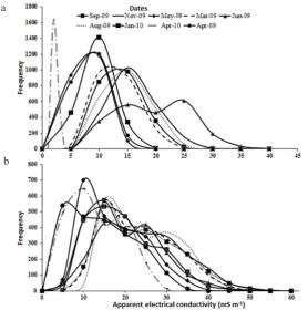
ECas produced unimodal distributions (except June
2009) and ECad were mildly bimodal (Fig. 6). For both
ECas and ECad, the months with the greatest cumulative
precipitation exhibited histograms slightly skewed to the right while the driest months were highly skew to the right,
indicating that the field should be mapped when soil water
content is near field capacity. June was the only ECas
data-set to have a bimodal distribution, supporting the inference that in that month, both depths experienced similar water and temperature conditions, which would also explain the
similar means for ECas and ECad.
Data for soil physicochemical properties are presented in Table 4. The soil samples were acidic with a mean pH
value of 4.4. ECe averaged 126.4 mS m-1 and ECa was
observed to increase with depth. Thus, ECas averaged
10.2 mS m-1 and ECa
d averaged 17.6 mS m-1. The
corre-lation coefficients between variables is shown in Table 5.
When the correlations of the soil properties and ECa were
explored, both ECad and ECas showed strong positive linear
correlation with clay-silt content (R = 0.67 and R = 0.78
respectively) and ECae (R = 0.76 and R = 0.60, respectively).
Although correlations of ECawith OM (ECad, R = 0.20;
Fig. 2. Mean shallow (ECas) and deep (ECad) apparent electrical conductivity (ECa) as functions of survey dates. Error bars are standard
error of the mean.
Visual inspection of the kriged clay-silt content map (Fig. 7), and kriged ECa maps (Fig. 5), showed remarkably similar spatial patterns where the south-western end of the
field had the lowest ECa and fine fraction values and the
north-eastern side had the highest. This distribution pattern suggested that high ECa readings were consistently found
in areas with finer texture, indicating that ECa can be used to interpret clay-silt content throughout the field site.
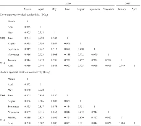
Spearman rank correlation coefficient was used to get
a quantitative measure of the time stability of spatial loca-tions between different mapping days (Table 2). The three wettest months (August, September and November 2009)
had the highest Spearman’s rank correlation coefficients
for both ECas and ECad. The highest occurred between
August 2009 and November 2009 (ECad) and August 2009
and September 2009 (ECas) with rs values of 0.97 and 0.95,
respectively. The fact that the correlations are high for the
wettest months surveyed, suggest similar ECas and ECad
responses with the increase in water content.
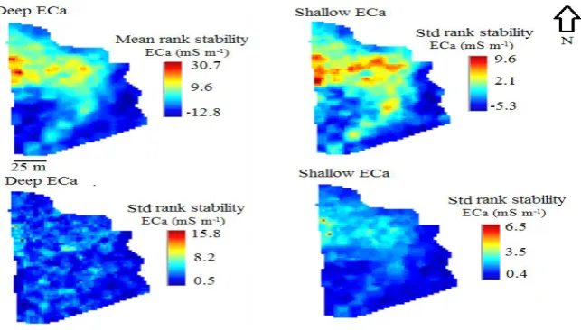
Figure 8 indicated locations that are consistently higher
than the field ECa average and locations that are consistent
-ly lower than the field average. The lowest ranked spatial
locations were 5.3 and 12.8 mS m-1 below the averaged mean
ECa of the nine mapping events for ECas and ECad,
respectively. While the highest ranked zones were 9.6
and 30.7 mS m-1 above the averaged mean for ECa
s and
ECad, respectively. The temporal stability maps do
indi-cate a general transition in soil texture across the field with
a combined decrease in ECe and clay-silt content from the
northern to the southern end of the field, as confirmed by
sampled soil. The textural variation may be as a result of
seasonal flooding of the study site. Beside leaching and temporary increases in soil electrical conductivity, flooding T a b l e 2. Spearman rank correlation coefficients deep (ECad) and shallow (ECas) apparent soil electrical conductivity
2009 2010
March April May June August September November January April
Deep apparent electrical conductivity (ECad)
2009
March 1
April 0.945 1
May 0.905 0.958 1
June 0.903 0.950 0.943 1
August 0.935 0.956 0.949 0.906 1
September 0.919 0.942 0.913 0.890 0.970 1
November 0.916 0.923 0.908 0.888 0.972 0.970 1
2010 January 0.914 0.939 0.938 0.927 0.957 0.932 0.954 1
April 0.919 0.946 0.943 0.927 0.925 0.919 0.919 0.949 1
Shallow apparent electrical conductivity (ECas)
2009
March 1
April 0.892 1
May 0.860 0.920 1
June 0.805 0.856 0.830 1
August 0.866 0.866 0.887 0.824 1
September 0.855 0.857 0.873 0.834 0.951 1
November 0.859 0.835 0.852 0.814 0.932 0.944 1
2010 January 0.819 0.823 0.862 0.824 0.870 0.867 0.922 1
ASSESSING THE TEMPORAL STABILITY OF SPATIAL PATTERNS USING GEOPHYSICS 429
Fig. 3. Correlation coefficients of monthly shallow vs. deep apparent electrical conductivity values in relation to cumulative monthly precipitation.
Fig. 4. Semivariograms for the kriged aparent electrical conductivity for (a) deep and (b) shallow data. All variograms were fitted with spherical models.
Cum
ul
at
iv
e m
on
th
lz p
re
ci
pi
ta
tio
n (mm)
C
oefficien
t o
f det
er
min
at
io
n (R
2)
a
b
R2
also redistributes soil sediments, by depositing the finest
textured soil closer to the river basin, drains and depressions
within the field. The standard deviation of the temporal sta
-bility map for the deep ECa measurements (Fig. 8) shows strong patterns. The locations of greatest change are
asso-ciated with particular features of the field, such as a small shed along the eastern field boundary and a network of deep drains in the center of the field, where leached salts
accumulated.
Both the shallow and deep ECa exhibited large-scale
similarly stable temporal patterns, thus both ECadepths can
be used to map the study site, however, since the feeder
roots of cocoa is located in the ECas range, ECas would
be better suited for soil management zone delineation. The results suggest that measurements of ECa patterns are inde-pendent of time and depth of measurement. Thus single
ECa mapping should suffice for the delineation of stable management zones in cocoa fields.
T a b l e 3. Variogram attributes ECad spherically fitted variogram models and ECas spherically fitted variogram models
2009 2010
March April May June August September November January April
Deep apparent electrical conductivity (ECad)
Nugget 0.07 0.03 0.08 0.04 0.05 0.06 0.05 0.01 0.03
Sill 1.06 1.16 0.98 0.90 1.02 1.02 1.15 0.91 1.30
Range 235.4 268.0 197.7 170.8 205.50 226.3 245.3 161.2 274.4
Shallow apparent electrical conductivity (ECas)
Nugget 0.14 0.09 0.13 0.07 0.13 0.10 0.11 0.03 0.12
Sill 0.63 0.94 0.68 0.52 0.57 0.45 0.60 0.48 0.68
Range 218.3 333.90 245.0 106.8 160.70 170.5 181.2 119.7 220.0
ASSESSING THE TEMPORAL STABILITY OF SPATIAL PATTERNS USING GEOPHYSICS 431
CONCLUSIONS
1. Our results showed a positive linear dependence of both shallow apparent soil electrical conductivity and deep apparent soil electrical conductivity on clay-silt content and soil solution electrical conductivity. Thus, apparent soil electrical conductivity signals can be used to interpret clay-silt content, soil solution electrical conductivity and delineate management zones.
2. The significant correlations between apparent soil
electrical conductivity and variables related to soil fertility such as organic matter, pH and gravimetric water content indicate that apparent soil electrical conductivity signals can also be used as soil fertility indicators.
3. Both the shallow apparent soil electrical con- ductivity and deep apparent soil electrical conducti- vity exhibited large-scale spatio-temporal pattern, thus both
Fig. 6. Frequency distributions of kriged apparent electrical conductivity (ECa) for the study site: a – ECa deep distribution and b – ECa shallow distribution.
T a b l e 4. Descriptive statistics of soil properties
Variable Mean Median deviationStandard Minimum Maximum Coefficient of variance (%)
ECad (mS m-1) 17.8 5.2 1.2 35.0 29.2
ECas (mS m-1) 10.2 10.1 2.9 4.6 19.3 28.4
θg (g g-1) 0.28 0.28 0.10 0.18 0.42 35.7
Clay-silt (%) 79.1 77.5 24.5 40.0 113.4 31.0
pH 4.4 4.4 0.4 3.4 6.7 22.6
ECe (mS m-1) 126.4 123.1 34.1 60.0 283.2 27.0
Organic matter (%) 2.5 2.4 0.6 1.0 3.1 22.1
ECad – deep apparent electrical conductivity; ECas – shallow apparent electrical conductivity; θg – gravimetric water content; ECe – soil solution electrical conductivity.
a
measurements would be suitable to delineate management
zones in cocoa fields in the humid tropic. If fields are to
be zoned based on the apparent soil electrical conductivi- ty measurements, however, shallow apparent soil electrical conductivity would be preferable, since the feeding roots of cocoa trees are concentrated in the upper 0.2 m of the soil. 4. The multi-mapping strategy using electromagnetic induction provides useful information for delineating soil textural boundaries without the costly and time demanding soil sampling, instrument calibration and remapping.
5. For non-saline soils planted with perennial crops such as cocoa, the thick organic litter and understory cover
cou-pled with humid tropical climate can minimize fluctuation
in transient properties (soil water and temperature) result-ing in apparent soil electrical conductivity signals that are time and depth independent.
T a b l e 5. Correlation matrix amongst soil properties in the study area
ECad (mS m-1) ECas (mS m-1) θg (g g-1) Clay-silt (%) pH ECe (mS m-1)
ECad (mS m-1) 1
ECas (mS m-1) 0.690 1
θg (g g-1) 0.278 0.250 1
Clay-silt (%) 0.673 0.783 0.274 1
pH 0.505 0.396 0.007 0.440 1
ECe (mS m-1) 0.763 0.603 0.158 0.473 0.634 1
Organic matter (%) 0.201 0.232 0.330 0.221 0.175 0.094
Explanations as in Table 4.
Fig. 7. Kriged spatial map of clay-silt % in the study site.
ASSESSING THE TEMPORAL STABILITY OF SPATIAL PATTERNS USING GEOPHYSICS 433
6. One mapping is enough to determine underlying
spa-tial patterns of properties related to soil fertility for efficient application of inputs and management of cocoa fields.
REFERENCES
Abdu H., Robinson D.A., and Jones S.B., 2007. Comparing bulk soil electrical conductivity determination using the DUALEM-1S and EM38-DD electromagnetic induction instruments. Soil Sci. Soc. Amer. J., 71, 189-196.
Atwell M., Wuddivira M., Gobin J., and Robinson D., 2013. Edaphic controls on sedge invasion in a tropical wetland assessed with electromagnetic induction. Soil Sci. Soc. Amer. J., 77, 1865-1874.
Bohling G., 2005. Introduction to geostatistics and variogram analysis. Available at: http://gismyanmar.org/geofocus/wp-content/uploads/2013/01/Variograms.pdf.
Bréchet L., Oatham M., Wuddivira M., and Robinson D.A., 2012. Determining spatial variation in soil properties in teak and native tropical forest plots using electromagnetic induc-tion. Vadose Zone J., 11, DOI:10.2136/vzj2011.0102. Burrough P.A. and McDonnell R.A., 1998. Principles of
Geo-graphical Information Systems. Oxford University Press, Oxford, UK.
Doerge T.A., 1999. Management zone concepts. Available at: http://www.ipni.net/publication/ssmg.nsf/0/C0D052F04A5 3E0BF852579E500761AE3/$FILE/SSMG-02.pdf. Eneje R.C., Asawalam D.O., and Ezemobi C., 2012.Variability
in physicochemical properties of some selected cocoa growing soils in Umuahia north local government area of Abia state. Res. J. Engr. Applied Sci., 1, 235-239.
Farahani H.J. and Buchleiter G.W., 2004. Temporal stability of soil electrical conductivity in irrigated sandy fields in Colorado. Trans. Amer. Soc. Agric. Eng., 47, 79-90. Gockowski J., 2007. Cocoa production strategies and the
conser-vation of globally significant rainforest remnants in Ghana. In: Production, markets, and the future of smallholders: the role of cocoa in Ghana. Inter. Inst. Trop. Agri., Accra, Ghana.
Goovaerts P., 2010. Geostatistical software. In: Handbook of applied spatial analysis. Springer Berlin Heidelberg, Germany.
Granger O.E., 1983. The hydroclimatology of a developing trop-ical island: a water resources perspective. Ann. Assoc. Amer. Geogra., 73, 183-205.
Haimelin R., 2008. Mapping soil water content on agricultural fields using electromagnetic induction. Report Helsinki Universty of Technology, Helsinki.
King J.A., Dampney P.M.R., Lark M., Mayr T.R., and Bradley R.I., 2001. Sensing soil spatial variability by electro-mag-netic induction (EMI): its potential in precision farming. In: Third European Conference on Precision Agriculture (Eds G. Grenier, S. Blackmore), Montpellier, France.
Lesch S.M., Strauss D.J., and Rhoades J.D., 1995. Spatial pre-diction of soil salinity using electromagnetic induction techniques 1. Satistical prediction models: Acomparison of multiple linear regression and cokriging. Water Resour. Res., 31, 373-386.
Mann K.K., Schumann A.W., and Obreza T.A., 2011. Delineating productivity zones in a citrus grove using citrus production, tree growth and temporally stable soil data. Prec. Agri., 12, 457-472.
Martinez G., Vanderlinden K., Ordóñez R., and Muriel J.L., 2009. Can apparent electrical conductivity improve the spa-tial characterization of soil organic carbon? Vadose Zone J., 8, 586-593.
Moral F.J., Terrón J.M., and Silva J.R., 2010. Delineation of management zones using mobile measurements of soil apparent electrical conductivity and multivariate geostatis-tical techniques. Soil Till. Res., 106, 335-343.
Nehmdahl H. and Greve M.H., 2001. Using soil electrical con-ductivity measurements for delineating management zones on highly variable soils in Denmark. In: 3rd Eur. Conf. Precision Agriculture, Montpellier, France.
Obalum S.E., Oppong J., Igwe C.A., Watanabe Y., and Obi M.E., 2013. Spatial variability of uncultivated soils in derived savanna. Int. Agrophys., 27, 57-67.
Remy N., 2005. S-GeMS: The Stanford Geostatistical Modeling Software: A Tool for New Algorithms Development. In: Geostatistics Banff 2004: 7th Int. Geostatistics Conf., Quantitative Geology and Geostatistics, September 26 - October 1, Alberta, Canada, Springer, the Netherlands. Rhoades J.D. and Chanduvi F., 1999. Soil salinity assessment:
Methods and interpretation of electrical conductivity meas-urements. FAO, 57, 1-150.
Robinson D.A., Lebron I., Kocar B., Phan K., Sampson M., Crook N., and Fendorf S., 2009. Time-lapse geophysical imaging of soil moisture dynamics in tropical deltaic soils: An aid to interpreting hydrological and geochemical pro-cesses. Water Resour. Res., 45, DOI: 2008WR006984. Rossi R., Amato M., Bitella G., and Bochicchio R., 2013.
Electrical resistivity tomography to delineate greenhouse soil variability. Int. Agrophys., 27, 211-218
Schumann A.W., Fares A., Alva A.K., and Paramasivam S., 2003. Response of ‘Hamlin’ orange to fertilizer source, rate and irrigated area. In: Proceedings of Florida State Horticultural Society, 116, 256-260.
Snoeck D., Abolo D., and Jagoret P., 2010. Temporal changes in VAM fungi in the cocoa agroforestry systems of central Cameroon. Agro. Sys., 78, 323-328.
Triantafilis J. and Lesch S.M., 2005. Mapping clay content variation using electromagnetic induction techniques. Comp. Elec. Agri., 46, 203-237.
Vachaud G., Passerat De Silans A., Balabanis P., and Vauclin M., 1985. Temporal stability of spatially measured soil water probability density function. Soil Sci. Soc. Amer. J., 49, 822-828.
Walter C., McBratney A.B., Douaoui A., and Minasny B., 2001. Spatial prediction of topsoil salinity in the Chelif Valley, Algeria, using local ordinary kriging with local va- riograms versus whole-area variogram. Aust. J. Soil Res., 39, 259-272.
Wood G.A.R. and Lass R.A., 1985. Cocoa. Longman Group Limited, London, UK.