Please cite this article as:S.M.A Hashemi, H. Haji Kazemi, A. Karamodin,Verification of an Evolutionary-based Wavelet Neural Network Model for Nonlinear Function Approximation, International Journal of Engineering (IJE), TRANSACTIONS A: Basics Vol. 28, No. 10, (October 2015) 1423-1429
International Journal of Engineering
J o u r n a l H o m e p a g e : w w w . i j e . i rVerification of an Evolutionary-based Wavelet Neural Network Model for Nonlinear
Function Approximation
S. M. A. Hashemi, H. Haji Kazemi*, A. Karamodin
Department of Civil Engineering, Ferdowsi University of Mashad, Iran
P A P E R I N F O
Paper history: Received 12April 2015
Received in revised form 14October 2015 Accepted 16 October 2015
Keywords:
Wavelet Neural Network Evolutionary Learning Algorithm Nonlinear Function Approximation
A B S T R A C T
Nonlinear function approximation is one of the most important tasks in system analysis and identification. Several models have been presented to achieve an accurate approximation on nonlinear mathematics functions. However, the majority of the models are specific to certain problems and systems. In this paper, an evolutionary-based wavelet neural network model is proposed for structure definition and optimization of nonlinear systems. The proposed model involves structure identification and also a parameter tuning phase to be adapted for modeling of an arbitrary system. The proposed structure and the learning algorithm are validated by comparing with some other most commonly used alternatives. The simulation shows the performance and adaptability of the proposed model in approximating multivariate nonlinear mathematics functions.
doi: 10.5829/idosi.ije.2015.28.10a.04
1. INTRODUCTION1
An important issue involved in system modeling is the identification of structure and function of a system. The aim of system identification is to identify a predefined simulation model that approximates a real world system [1-5] such as a controller. Hence, the process of system identification can be treated as a kind of function approximation. This process is commonly encountered in systems where a set of input-output pairs is also available. System identification has an extensive use in engineering problems, where the input output relationship is not linear. Some examples are: crack detection [6], the relationship between the input (Voltage and Velocity) and output (Force) in magneto-rheological (MR) dampers [4, 7], turbojet engines function [5], fuel cells functions [3] and some environmental cases [8]. Many more applications may be found in other references. Neural networks (NNs) have demonstrated great potential for system modeling even where the system dynamics is nonlinear [6, 9-12]. Lapedes and Farber [9] first proposed to use a
1*Corresponding Author’s Email: [email protected] (H. Haji Kazemi)
multilayer perceptron (MLP) neural network for nonlinear time series prediction. However, conventional neural networks process signals only on their finest resolutions.
The introduction of wavelet decomposition [7, 13, 14] provides a new tool for approximation. It produces a good local representation of the signal in both the time and the frequency domains. Inspired by both the MLP and wavelet decomposition, Zhang and Benveniste [8] proposed a wavelet network. This has led to the rapid development of neural network models integrated with wavelets. Most researchers have used wavelets as the basis functions that allow for hierarchical, multi-resolution learning of input-output maps from data.
WNNs have been used in the literature for approximation, classification, prediction and control problems [15, 16]. Unlike the sigmoidal functions used in conventional neural networks,wavelet functions are spatially localized, therefore the learning capability of WNN for system identification and control is more efficientthan the conventional sigmoidal function neural network. Thetraining algorithms for WNN typically converge more rapidly than those ofconventional NNs. Thus, WNN has been proved to be superior to the Gaussian-type neuralnetwork in that the structure can provide more potential to enrich the mapping relationship between inputs and outputs.
In this paper a Mexican-hat wavelet activation function neural network is used for chaotic function approximation. The proposed structure is optimized by an evolutionary algorithm. Structure definition and identification are described in section 2. Section 3 gives the results of implementation of the proposed method in comparison to some other methods. Finally some conclusions are drawn in section 4.
2. EVOLUTIONARY-BASED WAVELET NEURAL NETWORK MODEL
2. 1. Wavelet Neural Network Model The
proposed structure of the wavelet neural network is assumed to be a three-layer network comprising an input layer with nodes, a hidden layer with ̂ nodes, each having a wavelet activation function, and an output layer with nodes with a linear transfer function. A ̂ dimension weight matrix and a ̂ dimension vector are applied to the outputs of the first layer. A weight matrix of dimension ̂ will then be applied to outputs of the second layer and the row summation will be outputted for each node of the third layer. The mathematical operation of the network is described as follows.
Assume the input vector of as the th array set of dimension taken from the original set
{ } (1)
Then the input to the second layer will be
̂ ̂ (2)
where
̂ ̂ (3)
And
̂ { } ̂ (4)
in which ̂ and ̂ are the weights matrix and bias vector of first to second layer transit, respectively and ̂ is the number of neurons in the second layer.
Inputs of layer 2 have undergone the wavelet transfer functions, e.g. the Mexican hat as
(5)
while
̂ (6)
and
̂ (7)
in which is the output vector of the second layer and is the wavelet function. The outputs of the third layer can be calculated as
∑ ́ ̂ ̂
(8)
where ́ ̂ is the second to third layer weight matrix.
2. 2. Structure Identification To identify the structure of the constructed network a localized Genetic-based optimization algorithm is used. For a general optimization problem the aim is to minimize the objective function
(9)
(10)
where and refer to the ’th parameter and
optimum parameter set, respectively, in the network structure and is the total number of parameters.To achieve the minimum objective value, optimum structure of the network should be found. The optimum structure is subject to the optimum parameters set which is considered as the chromosomes after converted to binary format. A chromosome can be represented as
[ ]
(11)
For the structure described earlier, is the sum of the total number of weights, biases and wavelet parameters as
̂ ̂ ̂ ̂ ̂ (12)
The length of each chromosome will then be
̂ (13)
where is the resolution of real to binary conversion. Using Equation (13) one can estimate the size of the solution space of the problem by
̂ (14)
side, determines the enormousness of the solution space. Problems with more precise structure identification of desire require more efficient structure optimization algorithms. Operations of the genetic optimization algorithm are defined as follows. Reproduction operation selects a chromosome with the probability of
where for chromosome it is defined as
̇ ( )
̈
( )
(15)
in which ̇ and ̈ are the best network outputs (minimum objective values) gained in th generation and the total generations, respectively. It can be shown that for the best chromosome in each population . refers to the th selected chromosome through this operation and for the second selection, the last term in Equation (15) shows the coefficient of . This term constrains the number of chromosomes which are reproduced through this operation independent of their respective objectives. The second operation is defined as crossing over two or more qualified parents to create an intelligent offspring with inheritable features. In this operation to schemes of diversity preservation and good inheritance are embedded. Two or more parents, far from together, share their appropriate features to create a cross over offspring as
({ }
) (16)
where
( { ̇
})
̅̅̅̅̅( )
( {
})
(17)
in which and is the embedding function. Subscript determines the number of crossing parents which is chosen according to the dimension of the solution space. Parameter is initially set as √ ̂ . Refers to the probability of creation of the offspring for the next generation. Smaller values of will result in a higher probability of the cross over operation and vice versa. Equation (16) applies a higher probability of creation for the offspring which is better than the average of its parents and also the best chromosome in the th generation. The third operation is defined as the mutation operator which mainly turns around better chromosomes in each generation. A mutated offspring is created as
({ } ) (18)
where
̇ ( { })
̅̅̅̅̅( )
( { })
(19)
in which is the mutating function and since the probability of mutation operator is preferred to be lower that the probability of cross over operation. Some newly created chromosomes are transferred to the next generation according to their probability of creation. Some other chromosomes are also created to enroll the local search around the local optimum values. To this end, two operations are defined to trace the gradient of objective function in a discrete manner. The progressive operation is proposed as the fourth operation which is defined as follows
( ) ({ } ) (20)
where
( ) ( ) (21)
subject to
( ( )) ( ( )) (22)
while is the minimum possible parameter gradient regarding the conversion to binary. The probability of the progressive operation is the unit value which means for a preset of trials Equations (20) - (22) are retried iteratively to find a possible ( ).
If the search is not successful, subscript changes to its next value to search for another genome. Binary step size for the trials is a relatively short walk in the solution space random in all directions. The shareholder operation as the fifth operation is another localized search operation which creates a number of offspring by contributing randomly to select a genome from chromosomes and producing a chromosome from the selected genomes as
({ } ) (23)
where is the embedding function for the genomes randomly selected from individuals in the th generation. An assessment can be added to this operation to make it directive shareholder operations as
(
) ( ̇ ) (24)
3. SIMULATION RESULTS
In this section, the approximation capability of the evolutionary-based wavelet neural network (E-WNN) model for some benchmark mathematical functions is investigated. For the proposed model two validation processes are considered. First the structure is validated and then the structure identification algorithm is compared to other learning algorithms. In all validation processes the criterion will be the accuracy of nonlinear function approximation. To this end, four nonlinear multi-variable mathematical functions, commonly used as the benchmarks, are utilized to verify the convergence speed and structure optimization capability of the proposed model. The Mackey Glass time series is the first case of comparison. 1000 input-output data pairs as
[ ] (25)
are extracted from the following delay differential equation
(26)
For which and . This consideration means the embedding dimension and the lag are 4 and 6 respectively. The first 500 pairs are the training data set, while the remaining 500 pairs are the testing data set. The Rossler map is considered as the second case ̇
̇ ̇
(27)
where , for i=1, 2, 3 is the state variable of system, and
a, b, and c are positive constants which are set is this paper as a=0.15, b=0.2 and c=10. It is used in part as a chaotic function benchmark to test the model. In the Rossler map and the matrix of its first order partial derivative are estimated based on 1000 observations with the sample rate of 0.1. The third example is another well-known benchmark attractor named Lorenz attractor which is a three-dimensional continuous-time system
̇ ̇ ̇
(28)
where a, b and c are parameters and set to , and and the approximation is performed for 1000 observations.
As the forth function, one system can be described as
[ ] [ ] ( )
(29)
The model is identified in series-parallel mode defined as:
̂ ( ) (30)
It is a three-input–single-output fuzzy model. There are 200 input-target data sets chosen as training data. Another 200 input-target data in the interval are chosen as the testing data.
Table 1 shows the results of the experiment on evaluation of the proposed method in comparison with another commonly used models. Feed forward neural network as another structure is used to be trained by either Levenberg-Marquardt back propagation, Gradient descent back propagation learning algorithm or adaptive evolutionary learning algorithm. The wavelet neural network structure is also trained by either of the latter two. The model is validated in both structure identification and optimization. The criterion for function approximation has been selected as the mean square error (MSE) which is defined as follows
∑ ̅ (31)
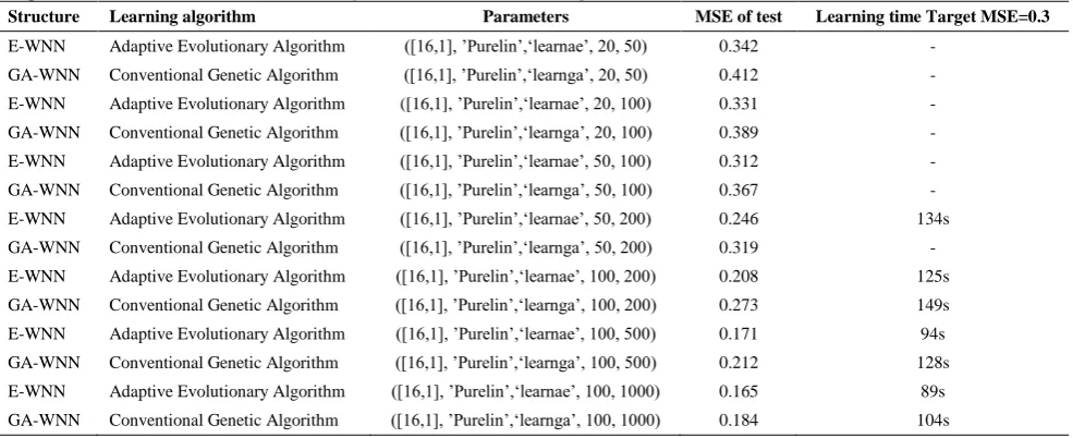
where and ̅ are real and desired outputs of the network, respectively, and N is the total number of samples. MSE of the testing samples indicates the system’s modeling capability. It can be seen from the results given in Table 1 that in the same running time of the models the wavelet neural network has better performance in nonlinear function modeling compared with the feed forward neural network while the same learning algorithm is used. However, Levenberg-Marquardt back propagation learning algorithm as a fast learning method require less time to reach a target value of the MSE but requires a much larger memory to process. It can also be inferred from the results of Table 2 that the adaptive evolutionary learning algorithm better tunes the parameters of the network structure while the network may be either a feed forward neural network or a wavelet neural network. From these discussions one can deduce that both the wavelet neural network structure and the adaptive evolutionary learning algorithm are superior to their competitors used in the experiments discussed in this paper.
response, the adaptive evolutionary algorithm reaches an optimized solution in a shorter time, compared to the conventional genetic algorithm. The results of Table 2
show how the adaptation of the genetic algorithm can improve it in terms of optimization capability and convergence speed.
TABLE 1. Comparison of the proposed model with some other models. For the proposed model Population=100 & Generation=up
to 500
Function Parameters MSE10 second MSE30 second MSE60 second TimeMSE:10-2 TimeMSE:10-3
S
tr
u
ct
u
re
i
d
en
ti
fi
ca
ti
o
n
Feed forward neural network structure + Levenberg-Marquardt back propagation
Function 1 ([16,1], ‘Logsig’,’Purelin’,‘Trainlm’) 0.212 0.207 0.203 91s 121s Function 2 ([16,1], ‘Logsig’,’Purelin’,‘Trainlm’) 0.315 0.311 0.309 94s 134s Function 3 ([16,1], ‘Logsig’,’Purelin’,‘Trainlm’) 0.114 0.108 0.107 87s 114s Function 4 ([16,1], ‘Logsig’,’Purelin’,‘Trainlm’) 0.367 0.356 0.351 97s 129s
Feed forward neural network structure + Gradient descent back propagation learning algorithm
Function 1 ([16,1], ‘Logsig’,’Purelin’,‘learngd’) 0.241 0.221 0.214 112s 153s Function 2 ([16,1], ‘Logsig’,’Purelin’,‘ learngd’) 0.363 0.334 0.331 123s 162s Function 3 ([16,1], ‘Logsig’,’Purelin’,‘ learngd’) 0.129 0.118 0.114 107s 124s Function 4 ([16,1], ‘Logsig’,’Purelin’,‘ learngd’) 0.385 0.373 0.367 145s 178s
WNN structure + Gradient descent back propagation learning algorithm
Function 1 ([16,1], ‘Mexicanhat’,’Purelin’,‘learngd’) 0.232 0.209 0.207 94s 129s Function 2 ([16,1], ‘Mexicanhat’,’Purelin’,‘learngd’) 0.337 0.324 0.321 99s 141s Function 3 ([16,1], ‘Mexicanhat’,’Purelin’,‘learngd’) 0.118 0.113 0.109 92s 118s Function 4 ([16,1], ‘Mexicanhat’,’Purelin’,‘learngd’) 0.381 0.371 0.359 112s 137s
Le
ar
n
in
g
a
lg
o
ri
th
m
v
al
id
at
io
n Feed forward neural network structure + Adaptive Evolutionary learning algorithm
Function 1 ([16,1], ‘Logsig’,’Purelin’,‘learnae’) 0.219 0.211 0.209 99s 145s Function 2 ([16,1], ‘Logsig’,’Purelin’,‘learnae’) 0.314 0.304 0.302 118s 159s Function 3 ([16,1], ‘Logsig’,’Purelin’,‘learnae’) 0.108 0.104 0.101 102s 121s Function 4 ([16,1], ‘Logsig’,’Purelin’,‘learnae’) 0.371 0.352 0.349 117s 146s
WNN structure + Adaptive Evolutionary learning algorithm
Function 1 ([16,1], ‘Mexicanhat’,’Purelin’,‘learnae’) 0.207 0.202 0.194 94s 127s Function 2 ([16,1], ‘Mexicanhat’,’Purelin’,‘learnae’) 0.311 0.303 0.301 101s 136s Function 3 ([16,1], ‘Mexicanhat’,’Purelin’,‘learnae’) 0.108 0.102 0.097 97s 118s Function 4 ([16,1], ‘Mexicanhat’,’Purelin’,‘learnae’) 0.345 0.332 0.327 109s 132s
*Logsig, Purelin and Mexicanhat are activation functions. **Trainlm, Learngd and Learnae are Training functions.
TABLE 2. Evaluation of the proposed model with different structural parameters ([Net size], Transfer function, Learning algorithm,
Population size, Generation size) for Mackey-Glass Time series modeling
Structure Learning algorithm Parameters MSE of test Learning time Target MSE=0.3
E-WNN Adaptive Evolutionary Algorithm ([16,1], ’Purelin’,‘learnae’, 20, 50) 0.342 -
GA-WNN Conventional Genetic Algorithm ([16,1], ’Purelin’,‘learnga’, 20, 50) 0.412 -
E-WNN Adaptive Evolutionary Algorithm ([16,1], ’Purelin’,‘learnae’, 20, 100) 0.331 -
GA-WNN Conventional Genetic Algorithm ([16,1], ’Purelin’,‘learnga’, 20, 100) 0.389 -
E-WNN Adaptive Evolutionary Algorithm ([16,1], ’Purelin’,‘learnae’, 50, 100) 0.312 -
GA-WNN Conventional Genetic Algorithm ([16,1], ’Purelin’,‘learnga’, 50, 100) 0.367 -
E-WNN Adaptive Evolutionary Algorithm ([16,1], ’Purelin’,‘learnae’, 50, 200) 0.246 134s
GA-WNN Conventional Genetic Algorithm ([16,1], ’Purelin’,‘learnga’, 50, 200) 0.319 -
E-WNN Adaptive Evolutionary Algorithm ([16,1], ’Purelin’,‘learnae’, 100, 200) 0.208 125s
GA-WNN Conventional Genetic Algorithm ([16,1], ’Purelin’,‘learnga’, 100, 200) 0.273 149s
E-WNN Adaptive Evolutionary Algorithm ([16,1], ’Purelin’,‘learnae’, 100, 500) 0.171 94s
GA-WNN Conventional Genetic Algorithm ([16,1], ’Purelin’,‘learnga’, 100, 500) 0.212 128s
E-WNN Adaptive Evolutionary Algorithm ([16,1], ’Purelin’,‘learnae’, 100, 1000) 0.165 89s
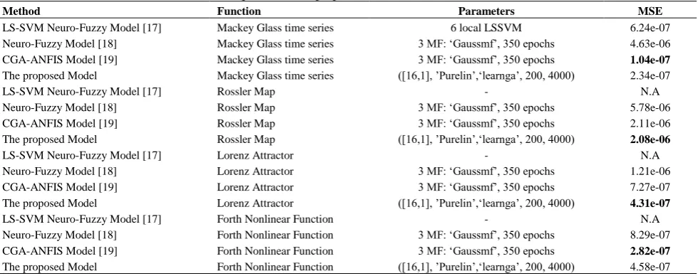
TABLE 3. Comparison of the proposed model with some other methods.
Method Function Parameters MSE
LS-SVM Neuro-Fuzzy Model [17] Mackey Glass time series 6 local LSSVM 6.24e-07 Neuro-Fuzzy Model [18] Mackey Glass time series 3 MF: ‘Gaussmf’, 350 epochs 4.63e-06 CGA-ANFIS Model [19] Mackey Glass time series 3 MF: ‘Gaussmf’, 350 epochs 1.04e-07 The proposed Model Mackey Glass time series ([16,1], ’Purelin’,‘learnga’, 200, 4000) 2.34e-07
LS-SVM Neuro-Fuzzy Model [17] Rossler Map - N.A
Neuro-Fuzzy Model [18] Rossler Map 3 MF: ‘Gaussmf’, 350 epochs 5.78e-06
CGA-ANFIS Model [19] Rossler Map 3 MF: ‘Gaussmf’, 350 epochs 2.11e-06
The proposed Model Rossler Map ([16,1], ’Purelin’,‘learnga’, 200, 4000) 2.08e-06
LS-SVM Neuro-Fuzzy Model [17] Lorenz Attractor - N.A
Neuro-Fuzzy Model [18] Lorenz Attractor 3 MF: ‘Gaussmf’, 350 epochs 1.21e-06 CGA-ANFIS Model [19] Lorenz Attractor 3 MF: ‘Gaussmf’, 350 epochs 7.27e-07 The proposed Model Lorenz Attractor ([16,1], ’Purelin’,‘learnga’, 200, 4000) 4.31e-07
LS-SVM Neuro-Fuzzy Model [17] Forth Nonlinear Function - N.A
Neuro-Fuzzy Model [18] Forth Nonlinear Function 3 MF: ‘Gaussmf’, 350 epochs 8.29e-07 CGA-ANFIS Model [19] Forth Nonlinear Function 3 MF: ‘Gaussmf’, 350 epochs 2.82e-07 The proposed Model Forth Nonlinear Function ([16,1], ’Purelin’,‘learnga’, 200, 4000) 4.58e-07
In order to compare the efficiency of the proposed model with other recently published methods this study implements the function approximation of four benchmark chaotic functions by LS-SVM Neuro-fuzzy model [22], Neuro-fuzzy model [23], CGA-ANFIS [24] and the proposed method. The results are given in Table 3 along with the parameters of the models. It can be seen that the proposed method outperforms the first two models for all benchmark functions. For two out of the four functions the proposed method attains a smaller error compared to the third method. It can be concluded that the proposed method yields better performance than the other methods in the approximation of the chaotic functions.
4. DISCUSSION AND CONCLUSION
In this paper a wavelet neural network was established in two phases. First the structure was constructed and then the parameters of the network were tuned by an adaptive evolutionary algorithm. The structure was described in details and the tuning process was also introduced. The proposed model was validated by comparing with other models commonly used in nonlinear function approximation. The experiments demonstrated the capability of the proposed model in the approximation of four nonlinear mathematics functions. Although the capability of the proposed model was validated in terms of modeling accuracy, the shorter learning times for the network may also be of interest. Therefore, for the future works the authors may seek other adaptation techniques for the genetic algorithm or try to combine the adaptive genetic algorithm with a fast convergent method to accelerate the convergence to the global optimum.
5. REFERENCES
1. Abiyev, R.H. and Kaynak, O., "Fuzzy wavelet neural networks for identification and control of dynamic plants a novel structure and a comparative study", Industrial Electronics, IEEE
Transactions on, Vol. 55, No. 8, (2008), 3133-3140.
2. Tzeng, S.T., "Design of fuzzy wavelet neural networks using the ga approach for function approximation and system identification", Fuzzy Sets and Systems, Vol. 161, No. 19, (2010), 2585-2596.
3. Sedighizadeh, M. and Kashani, M.F., "A tribe particle swarm optimization for parameter identification of proton exchange membrane fuel cell (technical note)", International Journal of
Engineering-Transactions A: Basics, Vol. 28, No. 1, (2014),
16-24.
4. Talatahari, S. and Rahbari, N.M., "Enriched imperialist competitive algorithm for system identification of magneto-rheological dampers", Mechanical Systems and Signal
Processing, Vol. 62, No., (2015), 506-516.
5. Tavakolpour-Saleh, A., Nasib, S., Sepasyan, A. and Hashemi, S., "Parametric and nonparametric system identification of an experimental turbojet engine", Aerospace Science and
Technology, Vol. 43, No., (2015), 21-29.
6. Deng, J., "Dynamic neural networks with hybrid structures for nonlinear system identification", Engineering Applications of
Artificial Intelligence, Vol. 26, No. 1, (2013), 281-292.
7. Khoa, T., Phuong, L., Binh, P. and Lien, N., "Application of wavelet and neural network to long-term load forecasting", in Power System Technology, 2004. PowerCon 2004. 2004 International Conference on, IEEE. Vol. 1, No. Issue, (2004), 840-844.
8. Zhang, Q. and Benveniste, A., "Wavelet networks", Neural
Networks, IEEE Transactions on, Vol. 3, No. 6, (1992),
889-898.
9. Lapedes, A. and Farber, R., Nonlinear signal processing using neural networks: Prediction and system modelling. Los Alamos
Nat. Lab Tech. Rep, LA-UR-872662. (1987).
10. Goharriz, M. and Marandi, S., "Assessment of lateral displacements using neuro-fuzzy group method of data handling systems", International Journal of Engineering-Transactions
11. Rakideh, M., Dardel, M. and Pashaei, M., "Crack detection of timoshenko beams using vibration behavior and neural network", International Journal of Engineering, Transactions
C: Aspects, Vol. 26, No. 12, (2013), 1433-1444.
12. Khalid, M., Yusof, R., Joshani, M., Selamat, H. and Joshani, M., "Nonlinear identification of a magneto‐rheological damper based on dynamic neural networks", Computer‐Aided Civil and
Infrastructure Engineering, Vol. 29, No. 3, (2014), 221-233.
13. SadeghpourHajia, M., Mirbagherib, S., Javidc, A., Khezria, M. and Najafpour, G., "A wavelet support vector machine combination model for daily suspended sediment forecasting"
International Journal of Engineering, Transactions C: Aspects
Vol.27, No.6 (2014), 855-864
14. Kim, H. and Adeli, H., "Wavelet-hybrid feedback linear mean squared algorithm for robust control of cable-stayed bridges",
Journal of Bridge Engineering, Vol. 10, No. 2, (2005),
116-123.
15. Wang, N. and Adeli, H., "Self-constructing wavelet neural network algorithm for nonlinear control of large structures",
Engineering Applications of Artificial Intelligence, Vol. 41,
No., (2015), 249-258.
16. Ganjefar, S. and Tofighi, M., "Single-hidden-layer fuzzy recurrent wavelet neural network: Applications to function approximation and system identification", Information
Sciences, Vol. 294, No., (2015), 269-285.
17. Miranian, A. and Abdollahzade, M., "Developing a local least-squares support vector machines-based neuro-fuzzy model for nonlinear and chaotic time series prediction", Neural Networks
and Learning Systems, IEEE Transactions on, Vol. 24, No. 2,
(2013), 207-218.
18. Razjouyan, J., Gharibzadeh, S., Fallah, A., Khayat, O., Ghergherehchi, M., Afarideh, H. and Moghaddasi, M., "A neuro-fuzzy based model for accurate estimation of the lyapunov exponents of an unknown dynamical system", International
Journal of Bifurcation and Chaos, Vol. 22, No. 03,
(2012),143-150.
19. Khayat, O., "Structural parameter tuning of the first-order derivative of an adaptive neuro-fuzzy system for chaotic function modeling", Journal of Intelligent & Fuzzy Systems, Vol. 27, No. 1, (2014), 235-245.
Verification of an Evolutionary-based Wavelet Neural Network Model for Nonlinear
Function Approximation
S.M.A. Hashemi, H.Haji Kazemi, A. Karamodin
Department of Civil Engineering, Ferdowsi University of Mashad, Iran
P A P E R I N F O
Paper history: Received 12 April 2015
Received in revised form 14 October 2015 Accepted 16 October 2015
Keywords:
Wavelet Neural Network Evolutionary Learning Algorithm Nonlinear Function Approximation
هديكچ
یکی یطخ ریغ عباوت بیرقت قیقد بیرقت روظنم هب یفلتخم یاهلدم .دشاب یم اه متسیس زیلانآ و صیخشت رد مهم دراوم زا
رد .دنا هدش فیرعت صاخ یاه متسیس و لئاسم یارب ،اهلدم نیا هدمع هک دنچ ره ،تسا هدش هئارا یضایر یطخ ریغ عباوت
یبصع هکبش کی هلاقم نیا
هنیهب و راتخاس نییعت روظنم هب یلماکت یکجوم هدش داهنشیپ یطخ ریغ یاه متسیس یزاس
یاه متسیس و عباوت یزاسلدم یارب راتخاس یاهرتماراپ میظنت و راتخاس ییاسانش مزیناکم کی زا هدش داهنشیپ لدم .تسا
اب هسیاقم قیرط زا نآ یارب هدش هتفرگ راک هب یشزومآ متیروگلا و یداهنشیپ راتخاس .دیامن یم هدافتسا هاوخلد یطخریغ
ریاس و ییاراک رگنایامن ،هدش ماجنا یاه یزاس هیبش .دوش یم یجنسرابتعا و ییامزآ یتسار لوادتم و لومعم یاهشور
.دشاب یم یضایر یطخریغ هریغتمدنچ عباوت بیرقت رد یداهنشیپ لدم ییاناوت