OPTIMIZATION OF TREE-STRUCTURED GAS DISTRIBUTION NETWORK USING ANT COLONY OPTIMIZATION: A CASE STUDY

(1)

IJE Transactions A: Basics Vol. 25, No. 2, April 2012 -141

OPTIMIZATION OF TREE-STRUCTURED GAS DISTRIBUTION

NETWORK USING ANT COLONY OPTIMIZATION: A CASE

STUDY

A. Mohajeri, I. Mahdavi*

Department of Industrial Engineering, Mazandaran University of Science and Technology, Babol, Iran [email protected], [email protected]

N. Mahdavi-Amiri

Faculty of Mathematical Sciences, Sharif University of Technology, Tehran, Iran [email protected]

R. Tafazzoli

Mazandaran Gas Company, Sari, Iran [email protected]

*Corresponding Author

(Received: March 08, 2011 – Accepted in Revised Form: December 15, 2011) doi: 10.5829/idosi.ije.2012.25.02a.04

Abstract An Ant Colony Optimization (ACO) algorithm is proposed for optimal tree-structured natural gas distribution network. Design of pipelines, facilities, and equipment systems are necessary tasks to configure an optimal natural gas network. A mixed integer programming model is formulated to minimize the total cost in the network. The aim is to optimize pipe diameter sizes so that the location-allocation cost is minimized. Pipeline systems in natural gas network must be designed based on gas flow rate, length of pipe, gas maximum pressure drop allowance, and gas maximum velocity allowance. We use the information regarding gas flow rates and pipe diameter sizes considering the gas pressure and velocity restrictions. We apply the Minimum Spanning Tree (MST) technique to obtain a network with minimum number of arcs, spanning all the nodes with no cycle. As a main contribution here, we present and use an ant colony optimization algorithm for solving the problem. The proposed method is applied to a real life situation. Our obtained results are compared to the ones obtained by an exact method. The results show that ACO is an effective approach for gas distribution network optimization. A case study in Mazandaran Gas Company in Iran is conducted to illustrate the validity and effectiveness of the proposed approach.

ﮑﭼ

ﯿ

هﺪ

،ﻪﻟﺎﻘﻣ ﻦﯾا رد زا

ياﺮﺑ نﺎﮕﭼرﻮﻣ يزﺎﺳ ﻪﻨﯿﻬﺑ ﻢﺘﯾرﻮﮕﻟا هدﺎﻔﺘﺳا ﯽﻨﺘﻧآ ﯽﻧﺎﺳرزﺎﮔ ﻪﮑﺒﺷ يزﺎﺳ ﻪﻨﯿﻬﺑ

ﯽﻣ

دﻮﺷ . ﯿﻬﺴﺗ ،ﺎﻫ ﻪﻟﻮﻟ ﯽﺣاﺮﻃ ﻪﻨﯿﻬﺑ ﯽﻧﺎﺳرزﺎﮔ ﻪﮑﺒﺷ ﮏﯾ ﯽﺣاﺮﻃ ياﺮﺑ يروﺮﺿ ﻒﯾﺎﻇو ﺰﺟ تاﺰﯿﻬﺠﺗ و تﻼ

ﺪﻧﻮﺷ ﯽﻣ بﻮﺴﺤﻣ .

يﺰﯾر ﻪﻣﺎﻧﺮﺑ لﺪﻣ ﮏﯾ ﻪﮑﺒﺷ رد ﺎﻫ ﻪﻨﯾﺰﻫ ﻪﯿﻠﮐ يزﺎﺳ ﻢﻤﯿﻧ ﯽﻣ رﻮﻈﻨﻣ ﻪﺑ ﻪﺘﺨﯿﻣآ ﺢﯿﺤﺻ دﺪﻋ

ﻪﺋارا دﻮﺷ ﯽﻣ . لﺪﻣ ﻦﯾا فﺪﻫ ،

ﯽﺑﺎﯾ نﺎﮑﻣ ﻪﻨﯾﺰﻫ يزﺎﺳ ﻢﻤﯿﻧ ﯽﻣ ﺎﺑ هاﺮﻤﻫ ﺎﻫ ﻪﻟﻮﻟ ﺮﻄﻗ هزاﺪﻧا يزﺎﺳ ﻪﻨﯿﻬﺑ -

ﺺﯿﺼﺨﺗ ﺪﺷﺎﺑ ﯽﻣ

. لﻮﻃ ،زﺎﮔ نﺎﯾﺮﺟ خﺮﻧ ﺮﺑ ﻖﺒﻄﻨﻣ ﺖﺴﯾﺎﺑ ﯽﻣ ﯽﻧﺎﺳرزﺎﮔ ﻪﮑﺒﺷ ﮏﯾ رد يراﺬﮔ ﻪﻟﻮﻟ ﻢﺘﺴﯿﺳ

ﺪﺷﺎﺑ زﺎﮔ زﺎﺠﻣ ﺖﻋﺮﺳ ﻢﻤﯾﺰﮐﺎﻣ و زﺎﮔ زﺎﺠﻣ رﺎﺸﻓ ﺖﻓا ﻢﻤﯾﺰﮐﺎﻣ ،ﻪﻟﻮﻟ .

ﺎﺑ ﻂﺒﺗﺮﻣ ﯽﺗﺎﻋﻼﻃا زا ،ﻪﻟﺎﻘﻣ ﻦﯾا رد خﺮﻧ

دﻮﺷ ﯽﻣ هدﺎﻔﺘﺳا زﺎﮔ رﺎﺸﻓ و ﺖﻋﺮﺳ يﺎﻫ ﺖﯾدوﺪﺤﻣ ﻦﺘﻓﺮﮔ ﺮﻈﻧ رد ﺎﺑ هاﺮﻤﻫ ﻪﻟﻮﻟ ﺮﻄﻗ هزاﺪﻧا و زﺎﮔ نﺎﯾﺮﺟ .

ندروآ ﺖﺳﺪﺑ ياﺮﺑ ﯽﺸﺷﻮﭘ ﺖﺧرد ﻢﻤﯿﻧ ﯽﻣ ﮏﯿﻨﮑﺗ زا ﻦﯿﻨﭽﻤﻫ هﺮﮔ ﯽﻣﺎﻤﺗ ﺶﺷﻮﭘ و لﺎﯾ ﻦﯾﺮﺘﻤﮐ ﺎﺑ يا ﻪﮑﺒﺷ

دﻮﺷ ﯽﻣ ﻪﺘﻓﺮﮔ هﺮﻬﺑ يا ﻪﺘﺴﺑ ﺮﯿﺴﻣ يﺮﯿﮔ ﻞﮑﺷ نوﺪﺑ ﺎﻫ .

ﻪﻟﺎﻘﻣ ﻦﯾا هﺪﻤﻋ ﻢﻬﺳ ﻪﻨﯿﻬﺑ ﻢﺘﯾرﻮﮕﻟا زا هدﺎﻔﺘﺳا رد

ﺖﺳا ﻞﯾﺎﺴﻣ ﻪﻧﻮﮔ ﻦﯾا ﻞﺣ ياﺮﺑ نﺎﮕﭼرﻮﻣ يزﺎﺳ .

زا هﺪﻣآ ﺖﺳﺪﺑ ﺞﯾﺎﺘﻧ زا هﺪﻣآ ﺖﺳﺪﺑ ﺞﯾﺎﺘﻧ ﺎﺑ ﻢﺘﯾرﻮﮕﻟا ﻦﯾا

ﺪﻧﻮﺷ ﯽﻣ ﻪﺴﯾﺎﻘﻣ ﻖﯿﻗد ﻞﺣ شور .

ﻢﺘﯾرﻮﮕﻟا ﻪﮐ ﺪﻨﻫد ﯽﻣ نﺎﺸﻧ ﺞﯾﺎﺘﻧ يدﺎﻬﻨﺸﯿﭘ

يدﺮﮑﯾور ،نﺎﮕﭼرﻮﻣ يزﺎﺳ ﻪﻨﯿﻬﺑ

ﯽﻣ ﯽﻧﺎﺳرزﺎﮔ ﻪﮑﺒﺷ يزﺎﺳ ﻪﻨﯿﻬﺑ ردﺮﺛﻮﻣ ﺪﺷﺎﺑ

. ﺖﺤﺻ ،نارﺪﻧزﺎﻣ نﺎﺘﺳا زﺎﮔ ﺖﮐﺮﺷ رد هﺪﺷ مﺎﺠﻧا يدرﻮﻣ ﻪﻌﻟﺎﻄﻣ

ﺪﻨﮐ ﯽﻣ ﺪﯿﯾﺎﺗ ار يدﺎﻬﻨﺸﯿﭘ دﺮﮑﯾور .

(2)

1. INTRODUCTION

Natural gas is one of the most important sources of energy. Exploration, extraction, production, and transportation are stages which natural gas goes through to secure consumers. The network contains three phases. The transmission of gas from central production facility to City Gate Station (CGS) is called a transmission phase, while forwarding gas from CGS to Town Board Station (TBS) is called a feeding phase. Securement of gas to consumers is performed in the distribution phase, where TBS is responsible for supplying the desirable gas pressure based on consumer’s viewpoint. Due to the movement of a large volume of gas at high pressures over long distances, transmission and distribution planning are basic elements of a natural gas network. While gas pressure is reinforced by compressors in the transmission network, it is reduced by pressure reduction stations in the distribution network. Gas pressure is lessened twice in the distribution network. CGS is defined as a pressure reduction station in which gas pressure is reduced from 1000 psi to 250 psi. In order to maintain the desired gas pressures based on consumers’ viewpoints, gas pressure should be fractured for a second time. A TBS is a pressure reduction station reducing gas pressure from 250 psi to 60 psi. Optimal types and locations of pressure reduction stations play key roles in minimizing the total cost in the network. Various topologies of natural gas network exist such as linear, structured, and cyclic. The tree-structured gas network is based on the minimum spanning tree (MST) model. This model is a combinational optimization problem. The model configures a connected graph with no cycles, spanning all the nodes in the network with the aim to minimize the total cost. This model has plentiful direct applications in computer design, telecommunication, transportation, pipeline network, etc. Also, indirect applications are in network reliability, clustering and classification problems.

The design of pipeline, facility, and equipment systems for securing consumers’ demands are necessary actions in the process of achieving an optimal natural gas network. There are factors influencing the total cost of a gas network such as pipe diameter, pressure, length, etc. Pipelines in a natural gas network must be designed based on gas

flow rate, length of pipe, gas maximum pressure drop allowance, and gas maximum velocity allowance. Gas minimum pressure allowance in the network is set to be 30 psi. In order to avoid the erosion phenomenon in a pipe, gas velocity should not exceed 20 m/sec. Consideration of all factors together for the design of an optimal gas network constitutes an impressive study. Gas companies usually apply heuristic methods which are based on human’s judgment and experience to find an optimal network. Trial and error procedures are common for such methods. But, for such methods to generate an optimal solution, one often needs an excessive computing work. Optimization methods, however, are suitable tools guaranteeing obtainment of optimal solutions with reasonable computing costs.

(3)

influencing the total investment of a gas network system (e.g. pipe diameter, thickness, pressure, length, compression ratio, etc). Hamedi et al. [2] presented an integrated multi-period optimization model for the distribution planning in different stages of natural gas supply chain. They formulated a mixed integer non-linear programming model with the aim to minimize direct or indirect distribution costs. In their work, a real-world case study of a natural gas supply chain was investigated. Optimization of gas transport in networks was investigated by Domschke et al. [3]. They considered networks containing pipes and various other components like compressor stations and valves with the aim to minimize the running costs of the compressor stations. Besides, they used different equations based on the Euler equation to formulate the gas flow through the pipes. Andre et al. [4] presented techniques for solving the problem of minimizing investment costs on an existing gas transportation network. They found the optimal location of pipeline segments to be reinforced and the optimal sizes and developed new heuristics for solving a non-linear problem. Numerous studies related to the case study on natural gas exist. Nørstebø et al. [5] optimized operation of the Norwegian natural gas system. GassOpt is a general tool for gas network optimization, but they applied it on the Norwegian gas transport network specifically. Erturk and Turut-Asik [6] analyzed the performance of 38 Turkish natural gas distribution companies by Data Envelopment Analysis (DEA). The results were used to detect the important criteria affecting the efficiency levels, and to find the common characteristics of the most inefficient firms. Our proposed natural gas network is focused on the gas distribution phase and is optimized by the Minimum Spanning Tree (MST) model and then is solved by a proposed ACO algorithm for large size problems. To solve optimization problems for gas networks, in recent years, several methods were developed and none of them have considered all aspects of the problem. The majority of them are based on the dynamic programming (DP) or gradient search techniques. The type of the methods used for solving optimization problems are influenced by problem’s nature. The work of Carter [7] represents one of attempts to optimize networks with general structures and with fixed

flow rates using DP techniques. Borraz-Sanchez and Haugland [8] proposed a solution method based on dynamic programming to address the fuel cost minimization problem to transport natural gas in a general class of transmission networks. They considered two types of continuous decision variables: mass flow rate along each arc and gas pressure level at each node and formulated a non-linear mathematical model. Wu et al. [9] formulated a model for fuel cost minimization. The model employs a gradient search technique for the gas network. Percell and Ryan [10] proposed a gradient search technique for minimization of fuel consumption in gas transmission networks.

The principal advantages of DP are that a global optimum is guaranteed and that the non-linearity can be easily treated. The disadvantages of DP are that its application is practically limited to the simple network topologies and that computation increases in an exponential way with problem dimension. The advantages of GRG method consist of that dimension is not a problem and, it could be applied to cyclic network schemes. However, as GRG method is based on a search gradient method, there is no guarantee to find a global optimum. In fact, with discrete decision variables, it can be fixed with the local optimum. The main original contribution proposed in this paper, is that we use the ant colony optimization (ACO) algorithm to solve our proposed natural gas network problem. The results obtained with the suggested approach are excellent with a strong computation time saving compared to those obtained with an exact method. This will enable us to design a fast, effective and robust decision aid tool based on the suggested method. This tool will assist operators to make the most appropriate decision within a short time.

(4)

colony algorithm to solve problems such as discrete optimization problems. Blum and Roli [12] investigated the ACO algorithm from an Operations Research (OR) viewpoint, classifying the algorithm as a metaheuristic one. Ant System (AS) was the first type of an ACO algorithm that was used for the Traveling Salesman Problem (TSP). This algorithm was introduced by Dorigo [13]. The ACO algorithm has plentiful applications to discrete optimization problems. Beside its use for the TSP problem, this algorithm is used for several other problems such as assignment, scheduling, graph coloring, and vehicle routing. Design of an ACO algorithm for MST problems was first proposed by Reimann and Laumanns [14]. The authors used the algorithm for the capacitated minimum spanning tree problems where capacity restrictions existed on the arcs. Complexity of gas network problems necessitates the employment of heuristic and metaheuristic algorithms. Chebouba et al. [15] optimized the natural gas pipeline transportation using an ACO algorithm. The authors proposed an ACO algorithm for the gas pipeline systems having fixed flow rate. The study focused on gas transmission networks where the compressor stations reinforced the gas pressure. The decision variables used in the study were the number of compressor stations and the amount of pressure discharged in each station. The aim of the proposed model was to optimize the consumed power in the network.

While most studies deal with transmission of natural gas, our study focuses on gas distribution networks. In recent years, some studies optimized pipe sizes in predefined structure of gas distribution networks. Conversely, we intend to construct an optimal gas distribution network having various pipe sizes along with the optimal types and locations of TBSs. Overall, our main original contribution proposed in this paper, is that we present the linear model to construct an optimal gas distribution network and propose the ACO algorithm to solve the large size problems. Here, we intend to conduct a case study of the natural gas network in Mazandaran Gas Company in Iran. The paper is organized as follows. A description of the natural gas network is given in Section 2. In Section 3, we present our proposed ACO algorithm. Section 4 discusses a case study conducted in Mazandaran Gas Company in Iran. Finally, conclusions are given in Section 5.

2. THE PROBLEM STATEMENT

2.1. Description Here, we focus on the gas

distribution phase of the natural gas network comprising of the pipelines having various sizes, TBSs, and consumers. The pipeline and TBS belong to the two indispensable components. The pipeline is responsible to connect the two places and to transmit a gas between them, while the TBS provides the motive force to maintain the natural gas flow through the network systems. The gas flow originates from the TBS and moves in a downward direction (i.e., it moves from a place with a higher pressure towards a place with a lower pressure). The amount of gas flow transferred between the two places is set to be the aggregate value of both demand and gas flow exited from a place with lower pressure. So, the consumers being farther away from the TBS have smaller pipe diameter size.

A gas distribution network is defined by the set of all nodes V and the set of all arcs A. In this network, consumers and the TBS are defined as a set of nodes and connected pipelines are defined as a set of arcs. A tree-structured natural gas network is described for the TBS and consumers. A tree is a connected graph with no cycles and all nodes spanned. Candidate locations for the TBS are given by the gas company. Our approach proceeds in two steps: (a) determination of the locations and types of the TBS, and (b) choice of the size of the pipelines. It is necessary to take into account several constraints. Some of these are restrictions of network infrastructure. Others are technical constraints such as the capacity constraints. We assume that pressure of gas should not be lower than 30 psi in the network. Also, the upper bound of gas velocity in the network is set to be 20 m/sec. Our model minimizes the total cost in the gas distribution network using the Minimum Spanning Tree (MST) technique.

2.2. Formulation This section presents a

(5)

cost values are calculated by gas company. This study uses the data available in the historical data of the company. The model is a single period planning tool used for short, medium, and long term planning.

A mathematical modelling of the gas transportation problem in networks was previously presented elsewhere. The model is general enough to take into account equations which govern the flow of the gas through pipes. The flow equation describes the relationship between pressure difference and gas flow in pipes. The relationship between pressure and flow rate exhibits a high degree of nonlinearity. In order to overcome this problem, we use the provided information based on the relationships among the gas flow rates and pipe diameter sizes by the gas company. They computed ratio of gas flow rates and pipe diameter sizes, keeping constant velocity and gas pressure. Velocity and gas pressure considered to be 20 m/sec and 30 psi, respectively. Table 1 shows the relationships among gas flow rates and pipe diameter sizes.

Here, a tree-structured gas distribution network is modeled efficiently using MST method. However, in order to guarantee the reliability of the gas system, a tree-structured network among the TBS is introduced into the pipeline network.

In this problem, the main objective in dealing with tree-structured pipelines is to determine the flow rate of pipelines in the network. As an impressive study, we show how to formulate the relationships among gas flow rates and pipe diameter sizes to minimize the flow cost. The model description follows here.

Notations:

I = set of candidate TBSs

T = set of TBS types

Z = set of consumer/demand zones

Parameters:

respect to the gas flow rate

t S z q it Q iz

d = distance between TBS i and consumer

zone z i

i d

'

zz d

consumer zone z' M Decision variables: i r     o.w. , 0 located is TBS if , 1 i it h     o.w. , 0 selected is type of TBS if ,

1 i t

itz y       o.w. , 0 type of TBS to connected is zone consumer if , 1 t i z z z w _        o.w. , 0 zone consumer to zone consumer between link direct a is there if , 1 z z i u     o.w. , 0 root a is TBS if , 1 i i i x _        o.w. , 0 TBS to TBS between link direct a is there if , 1 i i z

N =allocated number of consumers to

consumer zone z

i i

f _ = amount of flow from TBS ito TBS i'

z z

f = amount of flow from consumer zone z to consumer zone z'

z z

f  = amount of gas flow from consumer zone z

to consumer zone z'

z

ew = amount of congested gas flow to be

supplied to each consumer zone z

itz

w

e  = amount of gas flow from TBS iof type tto consumer zone z

Objective function:

min f  f₁ f₂f₃f₄ where, , 1 t I i t T

itS h

f



 

 (1)

,

2 y d C

f I i t T z Z

iz itz



    (2) , 3



      I i j J

i i i i d CT x

f (3)

.

4 w d C

f _z_z

Z z z Z

z z 

   



 

(4)

= distance between consumer zone z and

= a large number

= distance between TBS iand TBS i'

= capacity of TBS i of type t = demand of consumer zone z

= establishing the cost for TBS of type t unit among the TBS

(6)

Constraints:

, ,

i i

u r  i I (5)

, 1 



I i i u ₍₆₎



1



, , ,

i i ii

rM r x i iI (7)

, ,

, ii I

x

r_i _i_i   (8)



1





1 ,



,

ii i i

i I

x  u  M r i I





     



(9)



1





1 ,



,

ii i i

i I

x  u  M r i I

       



(10) , , ii i i I

x  r i I

    



(11) , , , ii ii

x f  i iI (12)

ii ii  (13)







u M 1

 

r 1



, i I, f

f _i _i

I i i i I i i

i        

     



(14)







1





1 ,



,

ii i i i i

i I i I

f  f  u M r i I



 



      



(15)

, ,

it i

t T

h r i I

   



(16) , , , itz it z Z

y h i I t T

     



(17) , , , itz it z Z

y h M i I t T



    



(18)

1 , ,

zz itz

z Z i I t T

w  y  z Z

  



   





(19)

1 , ,

z zz

z Z

N f  z Z









   (20)



1



, , ,

z zz zz

N M w   f z zZ (21)



1



, , ,

z zz zz

N M w   f z zZ (22)

, , ,

zz zz

f w M z zZ (23)

, , ,

zz zz

fw  z zZ (24)

zz z z zz  (25)

, , ,

1 M q ew f z z Z

w_z_z    _z  _z  _z_z   (26)

zz zz  (27)

, , ,

zz zz

fw  z zZ (28)

, ,

zz z

z Z

f  ew z Z



   



(29)



yitz1



M



qzewz



ewitz ,    i I, t T, z Z,(30)



y_itz1



M

 

 q_zew_z



ew_itz ,   i I, t T, z Z,₍₃₁₎

, , , ,

itz itz

ew y M      i I t T z Z (32)

, , , ,

itz itz

ew  y      i I t T z Z (33)

, , ,

itz it

z Z

ew Q i I t T

     



(34)

 

, , , , , , 1 , 0 , , , , , , Z z z T t I i i w x u y h

r_i _it _itz _i _i_i _z_z

           (35) . , , , , , 0 , , , , , Z z z T t I i i w e ew f f f

Nz ii zz zz z itz

              (36)

Equations (1)-(4) are the cost functions corresponding to the location-allocation costs. Constraint (5) indicates that exactly one TBS must be defined as a root. Constraint (6) ensures that there is exactly one TBS as the root in the network. Constraints (7) and (8) show the link between two TBSs. Constraints (9)-(11) impose that each TBS receive exactly one link from other TBSs if it is not the root node. The amount of flow between each TBS i and TBS i' is represented by constraints (12) and (13). Constraints (14) and (15) guarantee that there is no closed loop in the network. Constraint (16) shows that each TBS can adopt only one type when it is selected to service consumers. Constraints (17) and (18) ensure that each TBS covers at least one consumer. Constraint (19) represents that each consumer receives service from one consumer or one TBS. Constraint (20) determines the allocated number of consumers to consumer zones. Constraints (21)-(24) express the flow between two consumers. Constraints (25)-(28) represent the amount of gas flow from consumer zone z to consumer zone z'. Constraint (29) indicates the amount of congested gas flow for supplying other consumers by each consumer. The amount of gas flow from TBS to consumer is shown by constraints (30)-(33). Capacity restriction is shown by constraint (34). Constraint (35) imposes that the variables be binary. Non-negativity of the variables is represented by constraint (36).

f x M, i,i I,

f w M, z,z Z,

   

w 1 M q ew  f , z,z Z,









   

(7)

IJE Transactions A: Basics Vol. 25, No. 2, April 2012 -147 3. THE PROPOSED ACO ALGORITHM

Our proposed model is based on minimum spanning tree (MST) method which belongs to the NP-hard class of problem (Garey and Johnson, [16]). Because of the complexity of these problems, exact methods need excessive computation time. So, heuristic and metaheuristic algorithms are essential tools for solving such problems in reasonable amounts of time. However, such algorithms do not necessarily always find global optimum solutions, but yield good solutions in reasonable times.

From the optimization model, it can be discerned that our problem belongs to the discrete optimization problems. Since, the ACO algorithm has plentiful applications to discrete optimization problems (e.g. TSP problem, MST problem, Vehicle Routing problem, Network Routing problem, etc) and converges to solutions rapidly keeping quality of solutions, the optimization model is solved by a proposed ACO algorithm for large size problems. The ACO algorithm is proposed to attain near optimized solution, decrease computational complexity, and overcome the computer memory limitation.

3.1. Introduction Metaheuristic algorithms are

designed for solving optimization problems, taking their inspiration from nature. Dorigo [13] proposed an ACO algorithm to solve the combinatorial optimization problems.

The ACO algorithm is based on population and memory. A population-based approach produces different cycles in the algorithm. Each cycle contains a number of solutions. A memory-based approach saves the obtained information in each cycle. So, each cycle uses the obtained information in the previous cycles and gains solutions better than the previous ones. The algorithm cleans up the produced solutions at the end of each cycle.

In an implementation of an ACO algorithm consecutive, cycles are generated in which a number of solutions are produced by ants. At the end of each cycle, a pheromone trail matrix is updated using the obtained solutions. This process continues until the algorithm is terminated. There are essential elements to be considered in the design and implementation of an ACO algorithm. The elements are:

 A solution generation mode of ants.

 An updating mode for pheromone trail matrix.

 Stopping conditions.

3.2. A Solution Generation Mode A solution for

the tree-based natural gas network problem is composed of a tree which spans all nodes and has no cycle. In this structure, there exists a variety of candidate TBS combinations to secure consumers. Naturally, we are faced with networks with different sizes. So, each ant is responsible to produce a solution structure for each plan. First, each ant adopts a node from its set of TBSs and consumer nodes, randomly. Then, the next node is selected using a probability. The process continues until all the nodes are spanned. A solution structure is designed based on the following assumptions:

 There is at least one pipe exiting a TBS

 There is an uttermost nppipes exiting a TBS

 Connection links among the TBSs are tree-structured

The number of produced solution structures at the end of each cycle is to be equal to the number of different candidate TBS combinations.

3.3. A Selection Mode for Next Mode At first,

an initial node is selected by each ant, randomly. Then, each ant selects the other nodes using a transition probability function. This function allocates a transition probability to each node. To prevent construction of closed loops in the network, a list of nodes is maintained as a tabu list. A tabu list contains the nodes visited by an ant. A transition probability of nodes available in the tabu list is set to be zero. In contrast, the unvisited nodes constitute an allowed list of nodes for each ant. These are nodes not met previously by an ant. Let Tabu_k be the tabu list corresponding to ant k

and Allowed_kbe the allowed list of ant k. A

transition probability function is defined as follows:

(37)

 

   

   

 

 







otherwise, ,

0

, if

,

k k

ik ik

ij ij

ij

Tabu i Allowed j

t t

p

 

 



 

  

 





 





k Allowed

 

(8)

where, pij is the transition probability of node j corresponding to ant located at node i, _ijis set to

be 1d_ij with d_ij being the distance between nodes

iand j, _ij

 

t is the pheromone trail on arc

 

i,j in period t,  and are relative importance of

distance and pheromone trail, respectively.

Considering the selection mode for the next node, generation of infeasible solutions is possible. To prevent this, a solution structure should be adopted following the assumptions pointed out in the previous section.

3.4. An Updating Mode for Pheromone Trail Matrix Information is saved by the pheromone

trail matrix in the ACO algorithm. Updating of pheromone trail matrix at the end of each cycle is an essential task for the obtainment of new solutions. Let _ij

 

t be a pheromone trail on arc

 

i,j in period t. Each ant moves from the current

node to the next node in period t+1. An iteration is

defined as a movement of ant from the current position to another position. A tree structure is completed after n iterations. Note that n iterations

configure a cycle. Updating of pheromone trail on arcs at the end of each cycle is followed here:





 

,

ij t n ij t ij

       (38)

where, _ij

 

t is a pheromone trail on arc

 

i,j in period t,_ij



tn



is a pheromone trail corresponding to the similar arc in the next cycle,  is the resistance coefficient of pheromone trail, and so 1 is an evaporation rate of pheromone trail, and _ijis the pheromone trail on arc

 

i,j , secreted from each ant in interval



t,tn



, as specified below:

(39)

 





if ant uses arc , in

its tour between and

otherwise,

,

0, ij

i j

t t n

Q L

 

  

 _{ }

  

where, Q is a constant and Lis the length of the traveled path by ant at the end of each cycle.

We design a mutation operator to prevent

stagnation of the algorithm at the final step. After constitution of the updated pheromone trail matrix, each ant selects an arc, randomly. The pheromone trail corresponding to the arc is calculated as follows:

where,  is a mutation coefficient and N is the

total sum of number of TBSs and number of consumer nodes.

3.5. Stopping Condition Stopping condition can

be introduced in various forms. Here, our stopping condition for our proposed ACO algorithm is the maximum number of cycles allowed in the algorithm.

3.6. AlgorithmHere, the proposed ACO algorithm

is presented as follows.

Initialize maxiter, inittrail, ,,,. Set _i_,_j=inittrail, for all

 

i,j I,noiter0.

Generate a solution x using a construction

procedure.

Update the pheromone values and set x*x.

repeat

Compute xusing a construction procedure.

if f

 

x  f

 

x then

update the pheromone values. set x*x.

end if

noiter = noiter+1.

until stopping condition is met (i.e.,

noiter=maxiter)

Note that at the initial step, the parameters are initialized. Maxiter is used in the stopping condition for the proposed algorithm. Inittrail is an initial amount of pheromone trail for each arc. At the second step, a construction procedure is used to form a solution. Then, the pheromone trail matrix is updated and fitness function is evaluated. A fitness function for the proposed ACO algorithm contains two types of costs. The costs are:

(40)







 



 

N z

k

n t Max n

t ij

j i kz

1, interval the from

uniformly chosen

numbers random

, and with

, 1

,  

     

(9)

IJE Transactions A: Basics

 Establishing cost for TBS with respect to its type

 The cost of piping with respect to gas flow rate among the nodes

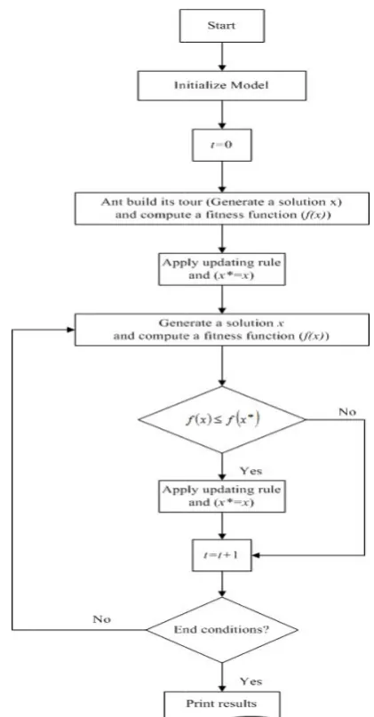
At the next cycles, if the fitness function is better than previous one, a pheromone trail matrix is updated. The main steps in the proposed ACO algorithm are shown in Figure 1 and include

 Ant builds its tour as it moves from one decision point to the next until all decision points have been covered

 The cost of the tour generated is calculated, pheromone is updated

 After the completion of one iteration (

fitness function is better than previous one, pheromone is updated.

A construction procedure of solution is given by Algorithm 2. This algorithm is tree

A tree is a connected graph with no spanning all the nodes with a minimal number of arcs.

(0) Give the input set of nodes V 



Set T 



tabu list



; A



set ofprobabilities



; 



P path

 

0_n

(1) Choose sVarbitrarily. (2) Set T 

 

s andA

   

V  s. (3) Compute R

 

_{ },

 

_{ }u,v

A v

v u

u 







 _



(4) Compute



.



 

T u

u R R

(5) Compute the probabilities:

 

   

  , , ,

,

, , ,

and .

u v u v

u v

u v u T v A

p u T v A

R

P P p

 

 

 

  _ 

   

    

  

(6) Find maximal probability value in

 

, max_{ }

 

, .

, * *

v u p v

u p

P v u p  

(7) Update the path matrix:

 

u*,v* 1.

path

(8) Update Tand A:

 

* ,  

 

* , .



T v A A v P

T

(9) If A then go to (3)

else, stop



thematrix path contains the

Vol. 25, Establishing cost for TBS with respect to its

The cost of piping with respect to gas flow At the next cycles, if the fitness function is better than previous one, a pheromone trail matrix is main steps in the proposed ACO

and include: Ant builds its tour as it moves from one decision point to the next until all decision The cost of the tour generated is calculated, fter the completion of one iteration (t), if the

fitness function is better than previous one, A construction procedure of solution is given This algorithm is tree-structured. A tree is a connected graph with no cycle, spanning all the nodes with a minimal number of



v1,v2,...,vn



;



allowedlist



; V





path matrix



. n

n



, uT.

, , ,

p     u T v A

Find maximal probability value in P:



. path optimal

Figure 1. Steps in the proposed ACO algorithm

Note that the minimum spanning tree approach makes use of a graph G= (V, E)

network, where Vis a set of nodes and

arcs. Tis a Tabu list and A

set of probabilities. The Path matrix contains 1 values. If each ant uses arc

related element is set to be procedure continues until all nod

the network. In other words, until the Allowed list for each ant becomes empty.

We now give an example to illustrate the steps of the above algorithm.

Example: Let V 



1,2,3,4,5



we have: T,

 

0₅_₅.



path

, No. 2, April 2012 -149

. Steps in the proposed ACO algorithm.

Note that the minimum spanning tree approach

G= (V, E) as a connected

is a set of nodes and Eis a set of

is an Allowed list. Pis a

The Path matrix contains 0 and If each ant uses arc

 

i,j in its tour, the related element is set to be 1; otherwise, 0. This procedure continues until all nodes are spanned in the network. In other words, until the Allowed list for each ant becomes empty.

We now give an example to illustrate the steps of



, following step (0),



1,2,3,4,5





A , P,

(10)

Step (1): Choose 4V. Step (2): T 

 

4 , A



1,2,3,5



.

Step (3): R₄

 

_{ }₄_,

 

_{ }₄_,_v , 4 T.

A v

v  









 _



Step (4): RR4.

Step(5):p(4,1) 0.25,p(4,2)0.35,p(4,3)0.10, (4,5) 0.30,

p 

and



₍₄_,₁₎0.25, ₍₄_,₂₎0.35, ₍₄_,₃₎0.10, ₍₄_,₅₎0.30



.

 p p p p

P

Step (6): p

 

*_,*  p_{ }₄_,₂ 0.35.

v u

Step (7): path_{ }4,2 1.

Step (8): T 

 

4,2 , A



1,3,5



, P . Step (9): Since A , Then go to step (3).

Step(3):

 

 

4,

 

 4, , 2

 

 2,

 

 2, .

4        v 

A v v v A v v R

R 



 





 

Step (4): RR₄R₂.

Step (5): p₍₄_,₁₎0.15,p₍₄_,₃₎0.15, p₍₄_,₅₎0.20,

p₍₂_,₁₎0.25, p₍₂_,₃₎0.15, p₍₂_,₅₎0.10,

and . 10 . 0 , 15 . 0 , 25 . 0 , 20 . 0 , 15 . 0 , 15 . 0 ) 5 , 2 ( ) 3 , 2 ( ) 1 , 2 ( ) 5 , 4 ( ) 3 , 4 ( ) 1 , 4 (                p p p p p p P

Step (6): p

 

*_,*  p_{ }₂_,₁ 0.25.

v u

Step (7): path_{ }2,1 1.

Step (8): T 

 

4,2,1 , A

 

3,5 , P . Step (9): Since A , Then go to step (3).

Step(3):  

 

 

 

 

 

   

 

  . , , , 1 , 1 1 , 2 , 2 2 , 4 , 4 4             v A v v v A v v v A v v R R R      



  

Step (4): RR4 R2R1. Step (5): p₍₄_,₃₎0.3,p₍₄_,₅₎0.05,

p₍₂_,₃₎0.2, p₍₂_,₅₎0.15,

p₍₁_,₃₎0.15, p₍₁_,₅₎0.15,

. 15 . 0 , 15 . 0 , 15 . 0 , 2 . 0 , 05 . 0 , 3 . 0 ) 5 , 1 ( ) 3 , 1 ( ) 5 , 2 ( ) 3 , 2 ( ) 5 , 4 ( ) 3 , 4 (                p p p p p p P

Step (6): p

 

*_,*  p_{ }₄_,₃ 0.3.

v u

Step (7): path_{ }4,3 1.

Step (8): T 



4,2,1,3



, A

 

5 , P . Step (9): Since A, Then go to step (3).

Step(3):  

 

 

 

 

 

   

 

  ,

 

 

 

  . , , , 3 , 3 3 , 1 , 1 1 , 2 , 2 2 , 4 , 4 4                 v A v v v A v v v A v v v A v v R R R R        



   

Step (4): RR4R2R1R3.

Step (5): p( 4,5) 0.3, p(2,5) 0.35, p(1,5) 0.15,

p₍₃_,₅₎ 0.2,

and



₍₄_,₅₎ 0.3, ₍₂_,₅₎0.35, ₍₁_,₅₎ 0.15, ₍₃_,₅₎0.2



.

 p p p p

P

Step (6): p

 

*_,*  p_{ }₂_,₅ 0.35.

v u

Step (7): path_{ }2,5 1.

Step (8): T 



4,2,1,3,5



, A , P.

Step (9): Since A , Then the algorithm stops

and we have: . 00000 01100 00000 01001 00000 5 5                  path

As many as different plans for candidate TBS combinations to secure consumers, the ants or solutions are formed. All ants are assumed to behave according to the above algorithms until convergence to solutions. The solutions are compared and the best is identified.

A natural gas network case study of Mazandaran Gas Company in Iran is conducted to verify the proposed model. Surveying on this case, nine

Iteration 1: and

Iteration 2:

Iteration 4:

Iteration 3:

(11)

potential locations for the TBS were decided. TBSs are selected to secure 119 consumers having definite demands. While the applied optimization software is not able to provide solutions for 119 consumers in a reasonable time, we categorized the customers into 11more comprehensive zones with aggregated demands. All the required information based on the relationships among gas flow rates and pipe diameter sizes are provided by the gas company. They computed ratio of gas flow rates and pipe diameter sizes, keeping constant velocity and gas pressure. Velocity and gas pressure were considered to be 20 m/sec and 30 psi, respectively. Table 1 shows the relationships among gas flow rates and pipe diameter sizes. Consumers’ demands are presented in Table 2. The total sum of consumers’ demands is 11195 m3_{/h. Three types}

of TBSs with different capacities exist in the network. Table 3 represents the establishing cost and capacity of different TBSs. We use the Minimum Spanning Tree (MST) technique to find a spanning tree in the network with a minimal total distance of the links. There are three types of connection links in the system.

Possible connection links are as bellow:

 Connection link between the TBS and consumer

 Connection link among TBSs

 Connection link among consumers

Tables 4-6 show distances corresponding to the defined connection links. The average cost of piping per distance unit among the TBS is considered to be 38000 units.

We applied CPLEX 11.0 software package to facilitate computations in our Mixed Integer Programming (MIP) model. CPLEX is a tool developed for solving large-scale linear optimization problems. It can also be used for quadratic programs. The available CPLEX optimizers are the standard primal simplex, dual simplex, network, barrier and mixed-integer optimizers [17].

Now, we make further experiments by changing the model to restrict the total number of pipes exiting a TBS by predefined values. For this, we need to change constraints (18) to:

, , ,

itz it z Z

y np h i I t T



     



(41)

where, np is the maximum number of exiting

pipes. We have used values of npequal to 2 and 3

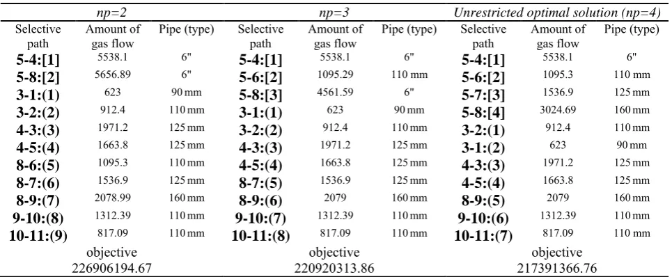
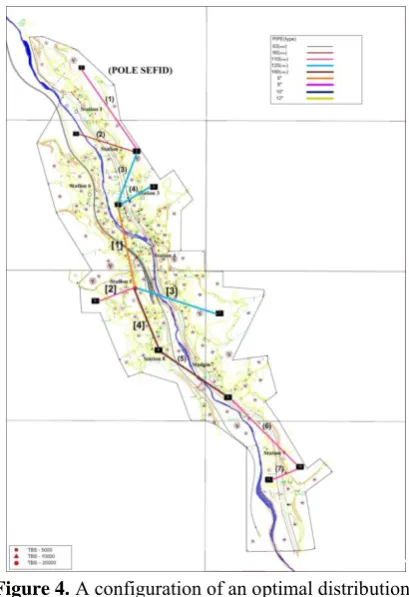
and reported the results in Table 7 along with the optimal solution obtained before, for comparison purposes. The validity of model is measured for gas distribution network case study of Mazandaran Gas Company in Iran as seen in Figures 2, 3, and 4, schematically. The results are summarized in Table 7. Table 7 presents objective function of three cases. As expected, the unrestricted case assures the global optimization and has the best objective function value i.e. the lowest cost. The objective function value in the np=2 and np=3

cases are little higher than the unrestricted case. Gas flow rates and pipe diameter sizes of selective paths are shown in Table 7. There are two types of connection links in the selective path column:

 Links connected between the TBS and consumers is indicated by a-b:[n] format; where, a and b indicate number of selected TBS and consumer, respectively. n is a number which indicates a selective path on the figure. [] is a symbol related to this kind of connection links.

 Links connected among the consumers is indicated by c-d:(n) format; where, c and d indicate number of selected consumers. () is a symbol related to this kind of connection links.

From Table 7, it is concluded that:

1. For np=2, np=3 and unrestricted case (np=4),

only one TBS of type three is selected (No. 5) to secure the total sum of consumers’ demands.

2. The aggregate value of gas flow in exiting pipes a TBS is equivalent to the total sum of consumers’ demands. That means, the whole of consumers’ demands in the network are met.

3. For np=2, two pipelines with the same

diameter sizes exit from the TBS (No. 5). 4. For np=3, three pipelines with different

diameter sizes exit from the TBS (No.5). 5. For unrestricted optimal solution (np=4), an

optimal gas distribution network with four pipelines exited from the TBS is reported in Table 7.

For np=2, np=3, and unrestricted optimal solution

(np=4), an optimal gas distribution network is

(12)

TABLE 1.The cost of piping per distance unit with respect to the gas flow rate

Gas flow rate (m3_/h) _{Pipe diameters (mm-inch)} _{Cost (unit)}

0-400 63 mm 11600

401-800 90 mm 14200

801-1500 110 mm 18500

1501-2000 125 mm 22000

2001-3800 160 mm 28000

3801-6000 6" 38000

6001-10000 8" 53000

10001-15000 10" 80000

15001-20000 12" 125000

TABLE 2.Consumers’ demands

CONSUMER 1 2 3 4 5 6 7 8 9 10 11

Demand(m3_/h) ₆₂₃ _912.4 _435.8 _1903.1 _1663.8 _1095.3 _1536.9 _945.7 _766.6 _495.3 _817.1

TABLE 3.The establishing cost and capacity of different TBSs

TBS types Capacity (m3/h) Cost (unit)

TBS 1 5000 50000000

TBS 2 10000 65000000

TBS 3 20000 85000000

TABLE 4.Distance among the TBS and consumers

D 1 2 3 4 5 6 7 8 9 10 11

1 160.854 363.9794 307.3191 813.182 888.1306 1515.165 1883.351 2027.984 2535.591 2990.097 3294.432 2 392.6576 736.3077 317.1577 417.0048 430.1093 1194.531 1433.087 1621.247 2098.236 2542.003 2857.911 3 758.0402 1127.865 690.0101 219.6952 114.3897 930.8501 1036.738 1252.259 1705.42 2145.709 2464.808 4 1218.117 1630.224 1195.905 533.0225 530.9652 643.1835 565.6925 756.1296 1204.854 1660.834 1964.456 5 1324.387 1789.507 1379.622 652.6354 777.5873 358.4983 626.2348 569.1696 1122.834 1615.072 1865.811 6 510.1853 1008.793 667.8877 240.3373 530.4988 861.3629 1322.241 1388.144 1927.745 2404.167 2679.914 7 2179.566 2605.866 2169.883 1491.181 1489.071 1054.943 509.5724 378.9512 242.6623 743.9207 993.0519 8 1919.088 2376.945 1956.269 1241.923 1306.719 710.2288 526.135 28.3196 581.3028 1086.803 1286.459 9 3096.335 3496.422 3052.351 2407.967 2360.768 1967.751 1336.361 1287.292 690.6902 239.8708 220.5176

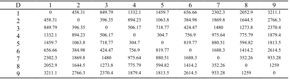
TABLE 5.Distance among the TBS

D 1 2 3 4 5 6 7 8 9

(13)

each pipe size. So, the selective paths given in Table 7 are indicated by different colors.

The objective function for unrestricted optimal solution is 217391366.76 units in 117573.93 seconds. Note that this computation time is needed to be spent for solving a problem with nine potential locations for the TBS and eleven consumer zones. Since, the real case at Mazandaran Gas Company in Iran contains 119 consumer zones with nine potential locations for the TBS, the applied optimization software is not able to provide solutions for 119 consumer zones

in a reasonable time. Due to the complexity of these problems, exact methods need excessive computation time. So, the ACO algorithm is an essential tool for solving such problems in reasonable amounts of time. However, such algorithms do not necessarily always find global optimum solutions, but yield good solutions in reasonable times. The test problems are produced to show the validity and effectiveness of our proposed algorithm. These problems are based on two factors (number of consumers and number of candidate TBS). Since the proposed model has

TABLE 6.Distance among the consumers

D 1 2 3 4 5 6 7 8 9 10 11

1 0 524.6723 370.6926 688.91 813.7481 1362.428 1777.473 1893.554 2415.647 2878.951 3172.612 2 524.6723 0 447.3679 1136.895 1138.036 1870.13 2160.459 2353.061 2833.109 3269.325 3592.613 3 370.6926 447.3679 0 734.0981 692.0065 1507.03 1715.998 1933.537 2393.807 2824.082 3152.555 4 688.91 1136.895 734.0981 0 334.0733 786.3078 1097.57 1217.516 1726.766 2192.192 2484.126 5 813.7481 1138.036 692.0065 334.0733 0 1018.077 1024.471 1286.822 1707.445 2132.091 2464.468 6 1362.428 1870.13 1507.03 786.3078 1018.077 0 940.0303 682.0594 1290.607 1796.184 1982.158 7 1777.473 2160.459 1715.998 1097.57 1024.471 940.0303 0 527.928 696.4919 1109.249 1444.573 8 1893.554 2353.061 1933.537 1217.516 1286.822 682.0594 527.928 0 609.2003 1114.753 1314.463 9 2415.647 2833.109 2393.807 1726.766 1707.445 1290.607 696.4919 609.2003 0 505.6095 759.6848 10 2878.951 3269.325 2824.082 2192.192 2132.091 1796.184 1109.249 1114.753 505.6095 0 421.2861 11 3172.612 3592.613 3152.555 2484.126 2464.468 1982.158 1444.573 1314.463 759.6848 421.2861 0

TABLE 7.Results for different np

np=2 np=3 Unrestricted optimal solution (np=4)

Selective path

Amount of gas flow

Pipe (type) Selective path

Amount of gas flow

Pipe (type) Selective path

Amount of gas flow

Pipe (type)

5-4:[1] 5538.1 6" 5-4:[1] 5538.1 6" 5-4:[1] 5538.1 6"

5-8:[2] 5656.89 6" 5-6:[2] 1095.29 110 mm 5-6:[2] 1095.3 110 mm

3-1:(1) 623 90 mm 5-8:[3] 4561.59 6" 5-7:[3] 1536.9 125 mm

3-2:(2) 912.4 110 mm 3-1:(1) 623 90 mm 5-8:[4] 3024.69 160 mm

4-3:(3) 1971.2 125 mm 3-2:(2) 912.4 110 mm 3-2:(1) 912.4 110 mm

4-5:(4) 1663.8 125 mm 4-3:(3) 1971.2 125 mm 3-1:(2) 623 90 mm

8-6:(5) 1095.3 110 mm 4-5:(4) 1663.8 125 mm 4-3:(3) 1971.2 125 mm

8-7:(6) 1536.9 125 mm 8-7:(5) 1536.9 125 mm 4-5:(4) 1663.8 125 mm

8-9:(7) 2078.99 160 mm 8-9:(6) 2079 160 mm 8-9:(5) 2079 160 mm

9-10:(8) 1312.39 110 mm 9-10:(7) 1312.39 110 mm 9-10:(6) 1312.39 110 mm

10-11:(9) 817.09 110 mm 10-11:(8) 817.09 110 mm 10-11:(7) 817.09 110 mm

objective objective objective

(14)

Figure 2.A configuration of an optimal distribution chain with two pipelines exited from the TBS

Figure 3.A configuration of an optimal distribution chain with three pipelines exited from the TBS

Figure 4.A configuration of an optimal distribution chain

been formulated for the case study of Mazandaran Gas Company in Iran, the generation of test problems are based on real data. Due to the limited capability of CPLEX 11.0 software package for solving our problems in a reasonable time, the test problems were produced in sizes convenient for the software to solve. The test problems are given as follows:

 One TBS and five consumers

 Two TBS and seven consumers

 Three TBS and six consumers

 Four TBS and nine consumers

 Five TBS and eleven consumers

(15)

Mutation coefficient

 

 : two levels (0.2-0.5).

Number of cycle (cyclenum): three levels (100-300-500).

Resistance coefficient

 

 : two levels (0.3-0.5).

Initial amount of pheromone trail (initial): two levels (50-100).

Relative importance of pheromone trail

 

 : three levels (1-3-5).

Relative importance of distance

 

 : two levels (2-4). There are232232144test plans. Each test plan is implemented for each defined test problem and the obtained results are saved using the following relation:

100,

ACO optimal optimal

f f

Gap f



  ₍₄₂₎

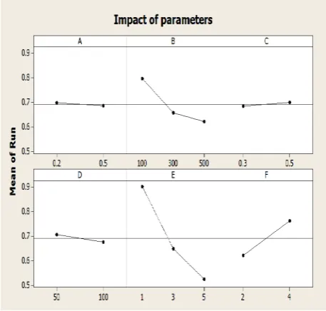
where, fACOis a fitness function of the proposed ACO algorithm and f_optimal is an optimal solution obtained by employing the exact method. The test problem’s gap is considered to compute the mean of gap for each test plan. Minitab 14.0 software package is applied to analyze the impact of different parameters on gap value. The results are shown in Figure 5.

Corresponding to the obtained results, levels 0.5, 500, 0.3, 100, 5, and 2 were selected for

 

 , (Cyclenum),

 

 ,(inittrail),

 

 ,and

 

 ,respectively.

4.1. Computational Results Here, the validity

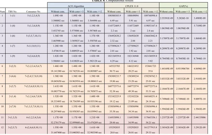
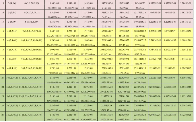
and effectiveness of the proposed ACO algorithm in comparison to the exact method is analyzed. The computational test was developed on a personal computer with Intel (R) Pentium (R) Dual with 2.2 GHz CPU / 4 GB RAM. The algorithm was coded using MATLAB R2009 software package. We considered five different problems for each test problem. Also, each problem contained three types (restricted to np=2, restricted to np=3, and

unrestricted). Consequently, we generated 75 test problems to test our proposed algorithm. The results are given in Table 8.

The results show that our proposed ACO algorithm is effective for solving the problems. The algorithm obtains good solutions in reasonable times.

In comparison to the exact method, the algorithm obtains solutions closer to the optimal solutions with much less time than the

Figure 5. Impact of each parameter on mean of gap

time needed to be spent for obtaining exact optimal solution.

The applied ACO approach in the real case at Mazandaran Gas Company in Iran provide 324645641 unit of cost while without the proposed mathematical model and the solution approach the cost was estimated by Mazandaran Gas Company's experts to be 625562000 unit of cost showing about 50 percent improvement.

5. CONCLUSIONS

(16)

contribution proposed in this paper, is that we presented the linear model to construct an optimal gas distribution networks having various pipe sizes along with the optimal types and locations of TBSs. In this paper, we used a MST technique to minimize location-allocation costs. Also, we constructed an optimal pipeline system considering various pipe diameter sizes. Advantage of our study was to acquire relationship among gas flow rates and pipe diameter sizes based on expert’s opinion and to show how to formulate it minimizing the flow cost. We used the actual data on Mazandaran Gas Company in Iran to conduct a case study. Optimal results were obtained applying CPLEX 11.0 software package. Due to the inability of this software to provide solutions for large size problems in a reasonable time, the ACO algorithm was proposed. The results obtained by the ACO algorithm were compared with those obtained by exact methods. Numerical results showed the effectiveness of the ACO algorithm for gas distribution network optimization. Therefore, the proposed ACO algorithm was applied in the real case at Mazandaran Gas Company in Iran having 119 consumers.

Finally, obtained results encourage us to study more complex structures (cyclic network topology). In this paper, it was assumed that the velocity and gas pressure are constant and the influence of them on the property of natural gas was neglected. The effects of these parameters on total cost were not included in the study, but would be continued in the future.

6. ACKNOWLEDGMENTS

We would like to give special thanks to Mazandaran University of Science and Technology and the Research Council of Sharif University of Technology. We would also like to thank the reviewers of the paper who made several constructive comments that helped improving the general content of the paper.

7. REFERENCES

1. Ruan, Y., Liu, Q. Zhou, W. Batty, B. Gao, W. Ren, J. and Watanabe, T., "A procedure to design the mainline system in natural gas networks", Applied Mathematical

Modelling, Vol. 33, (2009), 3040-3051.

2. Hamedi, M., Zanjirani, R.F. Moattar, M.H. and Esmaeilian, G.R., "A distribution planning model for

natural gas supply chain: A case study", Energy Policy,

Vol. 37, (2009), 799-812.

3. Domschke, P., Kolb, O. and Lang, J., "An adaptive model switching and discretization algorithm for gas flow on networks", Procedia Computer Science, Vol. 1,

No. 1, (2010), 1331-1340.

4. Andre, J., Bonnans, F. and Cornibert, L., "Optimization of capacity expansion planning for gas transportation networks", European Journal of Operational

Research, Vol. 197, (2009), 1019-1027.

5. Nørstebø, V.S., Rømo, F. and Hellemo, L., "Using operations research to optimize operation of the Norwegian natural gas system", Journal of Natural

Gas Science and Engineering, Vol. 2, (2010), 153-162.

6. Erturk, M. and Turut-Asik, S., "Efficiency analysis of Turkish natural gas distribution companies by using data envelopment analysis method", Energy Policy,

Vol. 39, (2011), 1426-1438.

7. Carter, R.G., "Pipeline optimization: dynamic programming after 30 years", Proceedings of 30th

PSIG annual meeting, (1998), 32-52.

8. Borraz-Sanchez, C., and Haugland, D., "Minimizing fuel cost in gas transmission networks by dynamic programming and adaptive discretization", Computers

& Industrial Engineering, Vol. 61, No. 2, (2011),

364-372.

9. Wu, S., Rios-Mercado, R.Z. Byod, E.A. and Scott, L.R., "Model relaxation for the fuel cost minimization of steady state gas pipeline networks", Mathematical and

Computer Modeling, Vol. 31, No. (2–3), (2000),

197-220.

10. Percell, P.B., and Ryan, M.J., "Steady-state optimization of gas pipeline network operation",

Proceedings of 19th PSIG Annual Meeting, (1987),

48-75.

11. Dorigo, M. and Stützle, T., "Ant Colony Optimization",

Series of Books in the Mathematics, MIT Press,

(2004), 305 pages.

12. Blum, C., and Roli, A., "Metaheuristics in combinatorial optimization: overview and conceptual comparison", ACM Computing Surveys, Vol. 35, No. 3, (2003), 268-308.

13. Dorigo, M., "Optimization, Learning and Natural Algorithms", Ph.D. Thesis, Dipartimento di Elettronica,

Politecnico di Milano, Italy, (1992).

14. Reimann, M., and Laumanns, M., "Saving based ant colony optimization for the capacitated minimum spanning tree problem", Computers & Operation

Research, Vol. 33, (2006), 1794-1822.

15. Chebouba, A., Yalaoui, F. Smati, A. Amodeo, L. Younsi, K. and Tairi, A., "Optimization of natural gas pipeline transportation using ant colony optimization",

Computers and Operations Research, Vol. 36, (2009),

1916-1923.

16. Garey, M.R., and Johnson, D.S., "Computers and intractability: a guide to the theory of NP-completeness", Series of Books in the Mathematical

Sciences, W.H. Freeman, (1979), 340 pages.

17. Vamanan, M., Wang, Q. Batta, R. and Szczerba, R.J., "integration of COTS software products ARENA & CPLEX for an inventory/logistics problem", Computers

(17)

TABLE 8.Computational results

ACO Algorithm CPLEX 11.0 GAP(%)

Num TBS No. Consumer No. Without cons. With cons<=3 With cons <=2 Without cons. With cons<=3 With cons <=2 Without cons. With cons<=3 With cons <=2 1 1-(1) 5-(1,2,3,4,5) 1.09E+08 1.09E+08 1.10E+08 108500385.9 108849094 109748998.4

2.55391E-09 5.2826E-10 3.4989E-09 3.580002 sec 3.560001 sec 3.564496 sec 6.49 sec 5.91 sec 6.97 sec

2 1-(4) 5-(1,3,6,8,9) 1.15E+08 1.15E+08 1.19E+08 114572469.5 114572469 119053167.4

1.06396E-08 1.06396E-08 5.7109E-09 3.452745 sec 3.575086 sec 3.587468 sec 2.2 sec 2 sec 2.4 sec

3 1-(6) 5-(3,5,7,10,11) 1.36E+08 1.36E+08 1.37E+08 136492630.2 136492630 136643042.8

5.17097E-09 5.17097E-09 1.8684E-09 3.465900 sec 3.569835 sec 3.550768 sec 2.32 sec 2.04 2.21

4 1-(7) 5-(1,5,8,9,11) 1.28E+08 1.28E+08 1.28E+08 127589624.7 127589625 127589624.7

5 1-(9) 5-(2,4,6,8,9) 1.82E+08 1.82E+08 1.82E+08 182136939.8 182136940 182136939.8

8.78458E-10 8.78458E-10 8.7846E-10 3.506841 sec 3.610820 sec 3.582128 sec 4.29 sec 4.12 sec 5.82

6 2-(2,5) 7-(1,2,3,4,5,6,7) 1.46E+08 1.48E+08 1.54E+08 145523703 146321852 153661723

1.44169E-09 0.931906784 4.8496E-09 18.141380 sec 18.742526 sec 18.803007 sec 30.73 sec 28.25 sec 35.6

7 2-(4,6) 7-(2,4,5,7,8,9,10) 1.58E+08 1.58E+08 1.59E+08 158309233.7 158309234 159250762.3

8 2-(3,7) 7-(3,5,6,8,9,10,11) 1.61E+08 1.61E+08 1.61E+08 160772573.6 160772574 160772573.6

9 2-(1,4) 7-(1,2,4,6,7,8,9) 1.52E+08 1.52E+08 1.60E+08 152182225.9 152182226 160160251.4

10 2-(7,9) 7-(1,3,5,7,9,10,11) 1.55E+08 1.55E+08 1.55E+08 155056996.4 155056996 155056996.4

11 3-(1,3,5) 6-(1,2,3,4,5,6) 1.17E+08 1.17E+08 1.21E+08 116935098.1 116935098 117665356.1 1.23572E-09 1.23572E-09 2.44135006

32.276179 sec 32.899660 sec 33.476269 sec 28.66 sec 34.99 sec 34.21 sec

12 3-(2,5,7) 6-(2,4,6,8,10,11) 1.55E+08 1.55E+08 1.61E+08 155292035 155292035 161277915.8 2.30342E-09 2.30342E-09 3.2912E-09

31.647400 sec 33.040303 sec 32.983540 sec 20.8 sec 26.01 sec 29.33 sec

<