Design, Modeling, Implementation and Experimental Analysis of 6R Robot (TECHNICAL NOTE)

TECHNICAL NOTE

DESIGN, MODELING, IMPLEMENTATION AND

EXPERIMENTAL ANALYSIS OF 6R ROBOT

M. H. Korayem*, R. Ahmadi, N. Jaafari, Y. Jamali and M. Kiomarsi

Department of Mechanical Engineering, Iran University of Science and Technology P.O. Box 16846, Tehran, Iran

[email protected]

A. Habibnejad

Department of Engineering, Tarbiat Modares University P.O. Box 14115-111, Tehran, Iran

[email protected]

*Corresponding Author

(Received: September 11, 2006 – Accepted in Revised Form: November 22, 2007)

Abstract Design, modeling, manufacturing and experimental analysis of a six degree freedom robot, suitable for industrial applications, has been described in this paper. The robot was designed on the assumption that, each joint has an independent DC motor actuator, with gear reduction and measuring sensor for angular joint position. Mechanical design of the robot was done using Mechanical Desktop and manufacturing process plan, the mechanical parts of the robot was developed. Kinematics and dynamics modeling of the robot was done using Mathematical and also MATLAB Robotics Toolbox and ADAMS software. The results from the kinematics and dynamics solution of the robot which was done mathematically, using Mathematical software, have been compared with the developed models of the robot, using MATLAB and ADAMS software for verification. An efficient geometric algorithm for the inverse kinematics problem of the robot was proposed. Finally, Experimental analysis and operational performance tests, including pose and path accuracy/repeatability of the robot's end-effecter, according to ISO 9283 standard was completed and the results are presented below.

Keywords 6R Robot, Dynamics, Kinematics, Design, Modeling, Manufacturing, Experimental Analysis, Test

ﻩﺪﻴﮑﭼ

ﺕﺎﺑﺭﻪﻧﻮﻤﻧﮏﻳﻲﻫﺎﮕﺸﻳﺎﻣﺯﺁﻱﺎﻫﺖﺴﺗﻡﺎﺠﻧﺍﻭﻱﺯﺎﺳﻝﺪﻣ،ﻲﺣﺍﺮﻃ،ﻪﻟﺎﻘﻣﻦﻳﺍﺭﺩ

ﯼﺍﺭﺍﺩ

ﻪﺟﺭﺩﺶﺷ

ﺖﺳﺍﻪﺘﻓﺮﮔﺭﺍﺮﻗﻲﺳﺭﺮﺑﺩﺭﻮﻣﻱﺩﺍﺯﺁ

.

ﻲﺣﺍﺮﻃﺯﺍﺲﭘﻭﺖﺧﺎﺳﺯﺍﻞﺒﻗ

ﺕﺎﺑﺭ

ﻱﺎـﻫﺭﺍﺰﻓﺍﻡﺮﻧﺭﺩﺕﺎﺑﺭﻱﺯﺎﺳﻝﺪﻣ،

ﺎﮑﻴﺘﻤﺘﻣﻭﺐﻠﻄﻣ،ﺰﻣﺍﺩﺁ

ﻡﺎﺠﻧﺍ

ﻩﺪﺷ

ﻴﻣﺎﻨﻳﺩﻭﻲﮑﻴﺗﺎﻤﻨﻴﺳﻱﺯﺎﺳﻪﻴﺒﺷﺞﻳﺎﺘﻧﻭ

ﺮﮕﻳﺪـﮑﻳﺎـﺑﺭﺍﺰـﻓﺍﻡﺮـﻧﻪﺳﺮﻫﺭﺩﻲﮑ

ﺖﺳﺍﻩﺪﻳﺩﺮﮔﻪﺴﻳﺎﻘﻣ

.

ﮊﺎـﺘﻧﻮﻣﻭﺖﺧﺎﺳﺯﺍﺲﭘ

ﻥﺩﺮـﮐ

ﻲـﺷﻭﺭ،ﺕﺎـﺑﺭ

ﯼﺍﺮـﺑ ﺶﻳﺎـﻣﺯﺁ

ﺖـﺳﺍﻩﺪـﻳﺩﺮﮔﻪـﺋﺍﺭﺍﻥﺁ

.

ﻲﻋﻮﻨﺘﻣﻲﻫﺎﮕﺸﻳﺎﻣﺯﺁﻱﺎﻫﺖﺴﺗ

ﺭﻮﻈﻨﻣﻪﺑ

ﺩﺭﺍﺪﻧﺎﺘـﺳﺍﺎـﺑﻖﺑﺎﻄﻣﺕﺎﺑﺭﻱﺩﺮﮑﻠﻤﻋﻱﺎﻫﻪﺼﺨﺸﻣﻦﻴﻴﻌﺗ

ﻭﺰـﻳﺍ ۹۲۸۳

ﺖﺳﺍﻩﺪﻳﺩﺮﮔﻡﺎﺠﻧﺍ

.

ﺞﻳﺎﺘﻧﺎﺑﺖﺴﺗﺞﻳﺎﺘﻧﻦﻴﻨﭽﻤﻫ

ﺕﺎـﺑﺭﻱﺩﺮـﮑﻠﻤﻋﻱﺎـﻫﻪﺼـﺨﺸﻣﻭﻪﺴﻳﺎﻘﻣﺕﺎﺑﺭﻱﺯﺎﺳﻪﻴﺒﺷ

ﺖﺳﺍﻩﺪﻳﺩﺮﮔﺵﺭﺍﺰﮔ

.

1. INTRODUCTION

Nowadays, the impacts of robots in industry are unquestionable, and robotic arms are implemented in most productive industries. Design and manufacturing of these robots and manipulators

freedom robot has been achieved by Ahmadi, et al [1]. This robot was designed and manufactured for lab tests. Sattari [2] has designed and manufactured a laboratory three degree freedom robot and also emphasizing on the importance of obtaining a proper dynamic model for robotic control; considers omitting the nonlinear terms in the torque equations of the system. Mokhtari [3] has designed and manufactured a 3P robot and kinematics analysis and simulation which were done considering optimization of choosing mechanical parts.

Liu et al. has introduced a system based on torque/force sensors for estimating the mass (inertia) parameters of the mechanical manipulator and their used estimated algorithm is based on Newton-Euler equations [4]. Taylon, et al [5] have developed and simulated a complete model of Scara robot. They have exploited equations of motions by using Lagrange dynamics and finally, operation of control system of actuators which was simulated, and approved by experimental tests. Some techniques for modeling and calibration have been done by Mottaa [6], using a measuring system based on three dimensional visions. Some of this system's properties were; being potable, cheap and accurate, also using a single camera. Experimental tests have been done for specifying the position accuracy of the two industrial robots; ABB IRB-2400 and Puma-5000 [6]. Modeling of Crs a251 industrial manipulator was done by Miro, et al [7] considering the motors specifications, kinematics and mass parameters. Dynamic equations of manipulator's motion have been solved using Lagrange method and Experimental analytical results were compared [7].

The earliest wrists were developed by Goertz [8] at Argonne National Laboratory for teleoperator handling nuclear materials. This device used sets of bevel gears for driving pitch and end effectors roll motion. The wrist had the singularity problem, which Raymond attempted by using additional spur gears to reduce the effect of the singularity [8]. Moritada, et al [8] invented a wrist with three degrees of freedom. Motors in the wrists forearm drives three parallel rotating shafts that terminate in spur gears. The central shafts connect to the wrist's body, rotating it for wrist roll. The upper shafts spur gear drives the large idler spur gear to decouple the upper shaft from

roll motion. Other attempts at wrist design and manufacturing include hydraulic servo mechanism by Rosheim [9]. These joints suffer because their hydraulic actuation has a slow time constant and can present the risk of explosion in certain environments. Colimitra [10] invented a wrist with three degrees of freedom which consists of hand gear train. This wrist in comparison with others is powerful and reliable. But the cost of manufacturing and controlling was the major difficulties of this wrist. Kung [11] presented a two degree of freedom spherical wrist for a robot. This design consisted of a spherical ball member with gear teeth formed in its outer surface and three drive gears that mated with the gear teeth in outer surface at 120 degrees division of rotation. By controlling the three drive gears to rotate by the proper amounts, the joint can be rotated about the desired axis of rotation. Rauchfuss [12] presented a wrist mechanism which access to any reachable point from any arbitrary direction. The wrist mechanism includes an intermediate joint created by two parallelograms, four bar linkage operating in parallel. This wrist only performs pitch motion. A new dexterous spherical wrist was presented by Wiitala [13]. The wrist consisted of a spherical eight bar closed loop linkage. It has five degree of freedom using the Gruebler Criterion [13].

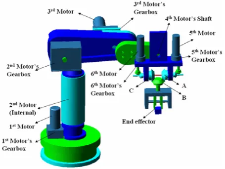
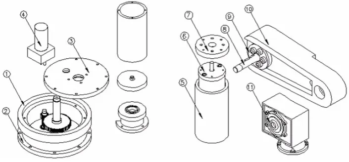
Figure 1. Schematic view of designed 6R robot.

2. DESIGN SELECTION OF 6R ROBOT

Proper configurations were accomplished by choosing a kinematics design with 6 degrees of freedom. Among the investigated designs, Cartesian, cylindrical, articulated and Scara manipulator design, can be mentioned. The final designed and manufactured robot that consists of six revolute joints is shown in Figure 1.

As it is seen, each joint has an independent DC motor actuator with gear reduction. The first link revolves around the vertical axis in horizontal plane, the second link revolves in vertical plane that is perpendicular to first link motion plane and the third and forth links in a plane parallel to the second link's motion plane. Fifth and sixth revolute motions are caused by a set of 45 degree bevel gears in the wrist mechanism. In the wrist mechanism altogether 7 bevel gears are entangled with each other simultaneously, four of them do the force transmission and three others are engaged with universal joint configuration. “A” and “B” gears are rotated by DC gearbox motors and the “C” gear as an output factor of motors is the actuator of the gripper which is linked to the set by the wrist adaptor. If “A” and “B” gears rotate with equal velocities and reverse directions the robot gripper will do just a roll movement. According to Figure 1 if “A” and “B” gears rotate with the same velocity and direction, the gripper just does the pitch motion. More complicated motions by this set can be achieved. So that if gear “A” is fixed (no rotation) and “B” rotates or vise versa “B” is fixed (no rotation) and “A” rotates then the gripper does the roll and pitch motions simultaneously. Briefly, it can be noted that, by creating difference in angular velocity of motors using the control unit simultaneous motion of pitch and roll can be achieved. Yaw movement can be achieved by another DC gearbox motor, directly coupled to the upper part of the wrist which in total three geared motors for three rotational motions of roll, pitch and yaw and combinational motions of roll and pitch has been designed. In this design, 38 parts has been used and there is possibility of installing different grippers, including 2 fingers or 3 pneumatic or suction fingers and aspiration grippers by the installing an adaptor on below the wrist. This adaptor has been installed in a way that the grippers have to be replaced by hand, but this adaptor has the

motions of roll and pitch, the ball bearings keep the center of rotation constant and the thrust ball bearing neutralizes the weight of the set.

3. MATHEMATICAL MODELLING OF THE 6R ROBOT

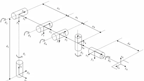
Kinematics and dynamics equations of this 6R robot are derived theoretically by using Denavite-Hartenberg parameters, as listed in Table 1. Complete description of coordinates and frames of this 6R robot is shown in Figure 2.

3.1. Direct Kinematics

parameters, kinematics for the robot is determined as follows [15]:

5 6 T 4 5 T 3 4 T 2 3 T 1 2 T 0 1 T

T = (1)

⎥ ⎥ ⎥ ⎥ ⎥ ⎦ ⎤ ⎢ ⎢ ⎢ ⎢ ⎢ ⎣ ⎡ = 1 0 0 0 z p z a z o z n y p y a y o y n x p x a x o x n

T (2)

where ) 6 S 234 S 6 C 5 C 234 C ( 1 C 5 S 1 S 6 C x

n =− + − (3)

6 S 234 S 1 S ) 5 S 1 C 1 S 5 C 234 C ( 6 C y

n = + − (4)

6 S 234 C 234 S 6 C 5 C z

n =− − (5)

) 6 S 5 C 234 C 234 C 234 S 6 C ( 1 C 6 S 5 S 1 S x

o = − + + (6)

6 S 5 S 1 C 1 S 5 C 234 C 4 23 S 1 S 6 C y o _⎟⎟ ⎠ ⎞ ⎜⎜ ⎝ ⎛ + −

= (7)

6 S 234 S 5 C 6 C 234 C z

o =− + (8)

5 S 234 C 1 C 1 S 5 C x

a =− − (9)

5 S 1 S 234 C 5 C 1 C y

a = − (10)

5 S 234 S z

a = (11)

)) 6 d 5 S 4 a ( 234 C 3 a 23 C 2 a 2 C 1 a ( 1 C 6 d 1 S 5 C x p − + + + + − = (12) ) ) 6 d 5 S 4 a ( 234 C 3 a 23 C 2 a 2 C 1 a ( 1 S 6 d 5 C 1 C y p − + + + + = (13) ) 6 d 5 S 4 a ( 234 S 1 d 3 a 23 S 2 a 2 S z

p =− − + + − + (14)

In order to verify forward kinematics equations, the results of robot forward kinematics that was determined by using Equations 12, 13 and 14, mathematically, is compared with the results of forward kinematics modeling, using MATLAB Robotics Toolbox and ADAMS. In this verification, the angular joint motion input, velocities and accelerations, which were done in 5 seconds, were determined by using Equations 15 to 20. Joints angular motion’s functions are as follows: 3 t 125 2 2 t 25 3

1= π − π

θ 0≤t≤5 (15)

3 t 250 2 t 100 3 2 π + π − =

θ 0≤t≤5 (16)

3 t 375 2 t 50

3= π − π

θ 0≤t≤5 (17)

3 t 250 2 t 100 3

4= π − π

θ 0≤t≤5 (18)

3 t 250 2 t 100 3 2

5 =−π+ π − π

θ 0≤t≤5 (19)

3 t 125 2 t 50 3 2

6=−π− π + π

θ 0≤t≤5 (20)

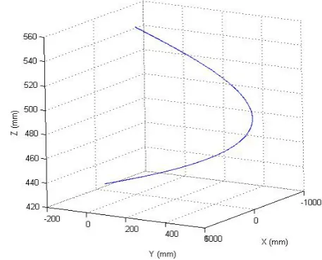
The end-effecter’s position which is related to the mentioned joint’s input is shown in Figure 3. [19]

3.2. Inverse Kinematics,

TABLE 1. Link Parameters of the 6R Robot.

Motion

θi

αi (˚)

di

ai

Joint Number (i)

Link 1

θ1

-90 d1 = 438 mm

0 1

Link 2

θ2

0 0

a2 = 251.5 mm

2

Link 3

θ3

0 0

a3 = 125 mm

3

Link 4 (Yaw)

θ4

90 0

a4 = 92 mm

4

(Pitch)

θ5

-90 0

0 5

(Roll)

θ6

0 d6 = 152.8 mm

0 6

Figure 2. Complete descriptions of 6R robot coordinate frames.

⎥ ⎥ ⎦ ⎤ ⎢

⎢ ⎣ ⎡

− − − = θ

x a 6 d x p

y a 6 d y p 1 tan

1 (21)

π + θ =

θ′_{1 1} (22) _⎥⎥

⎥ ⎥ ⎥ ⎥

⎦ ⎤

⎢ ⎢ ⎢ ⎢ ⎢ ⎢

⎣ ⎡

− ⎥⎦

⎤ ⎢⎣

⎡ _{− −}

± − = θ

1 S x p 1 C y p

2 1 2 ) 1 S x a 1 C y a ( 1 6 d 1 tan

Figure 3. The end-effecter's trajectory.

⎟

⎠

⎞

⎜

⎝

⎛

2 for

0

5 >

θ (24)

π + θ =

θ′234 234 for θ₅<0 (25)

⎥ ⎥ ⎦ ⎤ ⎢ ⎢ ⎣ ⎡ − − − = θ 1 S x n 1 C y n 1 C y o 1 S x o 1 tan

6 for θ5>0 (26)

π + θ =

θ′_{6 6} for θ₅<0 (27)

⎥⎦ ⎤ ⎢⎣ ⎡ − + ⎥ ⎥ ⎥ ⎥ ⎥ ⎥ ⎥ ⎦ ⎤ ⎢ ⎢ ⎢ ⎢ ⎢ ⎢ ⎢ ⎣ ⎡ ⎥ ⎦ ⎤ ⎢ ⎣ ⎡ − ± − = θ t u 1 tan 2 1 q w 2 ) q w ( 1 1 tan

2 (28)

2 2 C 2 a t 2 S 2 a u 1 tan

3 _⎥⎥−θ

⎦ ⎤ ⎢ ⎢ ⎣ ⎡ − − − =

θ (29)

3 2 234

4=θ −θ −θ

θ (30)

Where 234 C 4 a 234 C 5 S 6 d y p 1 S x p 1 C

t= + + − (31)

234 S 5 S 6 d 234 S 4 a 1 d z p

u=− + − + (32)

2 a 2 22 a 2 u 2 t 2 3 a

w= − + + + (33)

2 / 1 ) 2 u 2 t (

q= + (34)

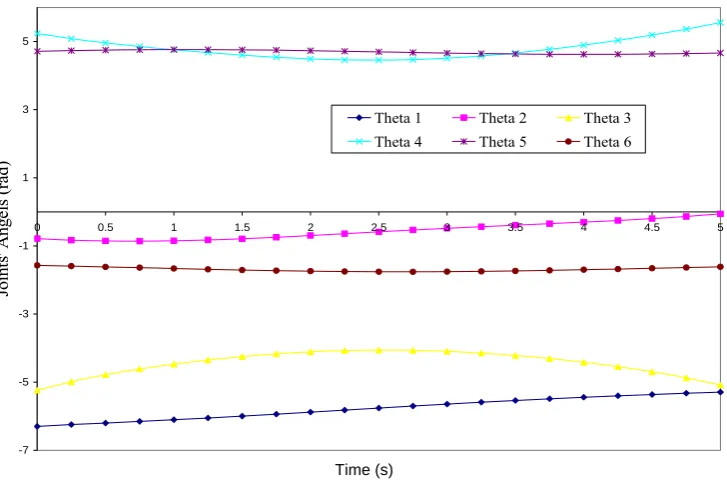
Verification of robot's inverse kinematics solution is done by comparing the results, which are obtained by the described algorithm in Equations 21 to 30, using Mathematical software versus the results which are obtained from the modeling of the robot in MATLAB Robotics Toolbox. Therefore the same linear trajectory of robot's end-effecter is applied as an input for the mathematical

algorithm of inverse kinematics, using Mathematical and also the model which is created in MATLAB software. The output results of six joints motions, using these two different methods are shown in Figure 4. The input is a linear trajectory between two points in the robot's workspace, at which the start point is the home position of the robot, as described in Table 2.

3.3. Dynamics Modeling of 6R Robot

equations of motion for an n axis robot manipulator are given by:

) ) t ( q ( b ) ) t ( q ( h )) t ( q ), t ( q ( c ) t ( q ) ) t ( q ( D ) t

( = && + & + + &

τ

(35) Dynamic equations of the 6R robot, based on

Equation 35, are derived by means of Lagrange-Euler method and also Newton-Lagrange-Euler method, using Mathematica software. Dynamic equations which were derived by these two individual methods are compared with each other. Results show that, equations which were derived by Newton-Euler formulation are the same as equations which was derived by recursive Newton-Euler formulation. Dynamics equations of this robot are very complex. The simplified dynamics equation for 5th _{joint which}

-7 -5 -3 -1 1 3 5

0 0.5 1 1.5 2 2.5 3 3.5 4 4.5 5

Time (Sec.)

Join

ts

' A

ng

els

(rad)

Theta 1 Theta 2 Theta 3

Theta 4 Theta 5 Theta 6

Figure 4. Motion of robot’s joints.

TABLE 2. Linear Input Trajectory for Inverse Kinematics.

X (mm) Y (mm) Z (mm)

Start Point 471.6 0 756.5

End Point 294.9 437.2 240.9

) 5 1 234 C )( 6 m 2 6 d

6 yy I 2 6 C 5 yy I 6 xx I 2 6 S ( )] 4 3 2 (

) 6 yy I 6 xx I ( 6 C 6 S 2 1 ) 4 a 234 C 3 a 23 C

2 a 2 C 1 a ( 6 m 6 d [ 5 S 2 1 ))] 3 2 ( 3 a 4 S

2 2 a 34 S ( 6 m 6 d 1 ) 6 yy I 6 xx I (

6 C 6 S 234 S 2 [ 5 C 2 1 234 S 5 C 6 m 6 gd 2 1 5

θ + θ +

+ +

+ θ + θ + θ

− −

θ −

−

− − +

θ + θ

+ θ −

θ −

+ =

τ

&& && && && & &

&& &&

&&

& & &

&

(36) The first term of the Equation 36, represents

loading due to gravity and other terms represent

inertia associated with the distribution of mass. The effect of friction is not considered in this robot's dynamic modeling.

Derived dynamics equations of the 6R robot in Mathematica, is compared with dynamics simulation results of the robot modeling, using MATLAB Robotics Toolbox and ADAMS. Joint torques required to achieve the specified state of joint position, velocity and acceleration, is computed with derived dynamic equations, using Mathematica and also determined from simulation results of the robot model, using MATLAB Robotics Toolbox and ADAMS software. Joint torques for the joint space trajectory, which is mentioned in Equations 15 to 18, is shown in Figure 5.

-0.7 -0.5 -0.3 -0.1 0.1 0.3 0.5

0 1 2 3 4 5

Time (Sec.)

T

o

rq

u

e

o

n

Joi

nt 1.

(

N

.m

)

Mathematica MATLAB ADAMS

0 1 2 3 4 5

Time (Sec.)

T

o

rqu

e on Joi

nt

2.

(

N

.m

)

Mathematica MATLAB ADAMS

5.3 5.4 5.5 5.6 5.7 5.8 5.9

0 1 2 3 4 5

Time (Sec.)

T

o

rq

u

e on Joi

nt

3.

(

N

.m

)

Mathematica MATLAB ADAMS

0 1 2 3 4 5

Time (Sec.)

T

o

rq

u

e

on

Joint 4.

(

N

.m

)

Mathematica MATLAB ADAMS

Figure 5. Actuator torque at the joints.

4. ROBOT OPERATION AND TECHNICAL POINTS OF MANUFACTURING AND

ASSEMBLING

One of the most important features of this robot is designing the links drive system to be directly coupled with the links through speed reduction gearboxes. This configuration of design is highly accurate and eases assembling or disassembling. Five motors of this robot are geared motors. In the first and third links, the output speed of geared motors is again reduced through couple of gears. Selections of proper bearings have been considered in robot’s mechanical design and as a result, it will directly affect the robot's accuracy. Mechanical parts of the robot are described in Figure 6. One of

the manufacturing points of the first link, is the application of aluminum as the gearbox housing material (part number 1) which causes the weight decrease, easy to machine, and a good appearance, provided that an accurate and proper machining is being done. The material used for the bottom and the lead (cap) parts of gearbox housing is stainless steel and the reason for this choice is that the housings bearing machined on these two parts won't loose its dimensional accuracy because of several assemblies and disassemblies which may be needed. As a result, an accurate assembly for the bearings and shafts, of the gearbox will be possible. Another point that can be mentioned is that the stainless steel used for the mentioned parts (parts number 2 and 3) is of ferrite kind because

Time (s) Time (s)

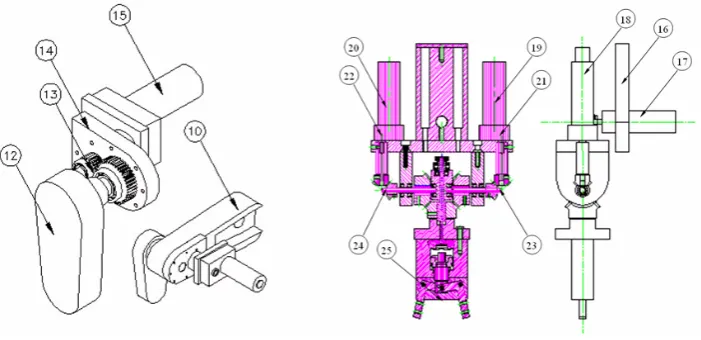
Figure 6. Mechanical parts of the 1st and 2nd links.

the austenite kind can't be magnetized and therefore it can't be honed by using honing machine which holds the part with magnetic force and for this reason, the ferrite steel was chosen, as a result, the surface of the honed parts was accurately parallel, therefore the assembly was accurate. The second link (part number 10), revolves in a plane perpendicular to the working plane of the first link and revolves in a 270 degree range though this range is not necessarily used. Using a gearbox (Part number 11) for power transmission with worm and gear structure makes a 90 degree difference in the output and input shaft; hence, orientation of the second link in vertical plane will be possible. The input axis of the motor (Part number 6) is co-axial with the first link, so by designing the first link in the form of a hollow cylinder, the motor of the second link designed to be assembled in this hollow cylinder and as a result, this design made the workspace of robot wider and also gave a good appearance to the robot. Since the second link joint is the most important joint of the manipulator from the imposed torque point of view, so for imposing such a torque on the link of the second joint, a gearbox (the worm and gear gearbox explained before) with 1:100 gear ratio was used. The motor coupled to this gearbox has a high torque with 1600 rpm. The torque of the output shaft of gearbox of the second link is transmitted to the second link via a flange coupling. As the gearbox ratio is 1:100, the output torque of the gearbox of

the second link will be proper and sufficient for a soft revolution, although there is heavy load on the link (about 11 kg including the second link, third link, wrist without considering the external load that the robot grips and loads).

One other point that should be mentioned is, the gearbox of the second link is a self locking gearbox because of the geometry and mechanics of the worm and gear engagement, this makes it beneficial because the second link always remain in the stop position with high accuracy.

The material used for the second link was aluminum and made in the form of “T” which makes them resistant to strains and at the same time this feature makes robot to be accurate. As we get closer to the end of the link, the cross section area of the link linearly decreases as we get near the end, where this feature helps to have the optimum design for the link, also prevents unnecessary increase of the link's weight and to keep it at minimum. The resistant torque exerting on the joint is with the maximum moment of inertia.

Figure 7. Mechanical parts of the 3rd, 4th, 5th and 6th links.

and bearings which has been deliberately designed, machined and assembled in the accurately machined housing at the end of the second link. This pinion and gear assembly transmits the power to the third link and because of the ratio between these two gears; the output torque of the geared motor of the third link nearly doubles. The geared motor of the third link (Part number 15) is assembled on the second link by an adaptor part (part number 14) and its output shaft is coupled to the pinion inserted in the machined housing of the second link [16].

The output torque of the gear is transmitted to the third link by using a flange, coupled to the third link. The wrist of the robot is attached to the third link, which can resolve in a 270 degree range. In order to introduce a wrist design, we will investigate the wrist assembly which also includes a pneumatic gripper as shown in Figure 16, the wrist design consists of three shafts, seven gears, three coupling, four bases, a main base for assembling motors, adaptor, seven ball bearings, one thrust ball bearing, a number of screws and retaining keys, etc. Motor number 17 as shown in Figure 7 can rotate the whole structure of the wrist and acts as a fourth joint. Motors number 19 and 20 through their reduction gearboxes (Parts number 21 and 22) generates the pitch and roll motions of the robot’s end effector. The bases of spherical (ball) joints have been designed so that assembling and disassembling, can be done with

optimum accuracy as the first assembly; this is made possible by using male on the bases. The available adaptor in design makes the installation of different grippers possible [17]. Figure 8 shows the manufactured manipulator is assembled with the wrist and gripper.

5. EXPERIMENTAL ANALYSES AND PERFORMANCE TESTING

The robot should accomplish the given commands accurately and smoothly. This is possible only if the end effector is accurate relative to the work piece. The robot's accuracy is under the effect of the following factors:

• The accuracy of manufacturing mechanical parts of the robot.

• The accuracy of assembling the constituting parts of robot.

• Accuracy during the robot operation which is influenced during the by external forces.

• Electronic systems accuracy and motor's motion.

• The existing clearance in the system.

• Wear behaviors, which change the accuracy of robot in long duration.

In order to reach logical and desired accuracy, all above mentioned items have to be carefully attended. In order to have an accurate robot (a robot with high accuracy) all matters related to manufacturing and quality control of all parts must be accurately considered and controlled according to the drawings with proper geometrical and dimensional tolerances, specified in design. The robots posed accuracy and repeatability is measured according to the ISO 9283 standard, which was done for the robot as follows [18]:

5.1. Position Accuracy

accuracy, the robot is given command for “n” times to go to certain point xc, yc, zc and the

coordinates xj, yj, zj is obtained by calculation of

the following equations, by which we reach the position accuracy (APp):

) c z z ( z AP ), c y y ( y AP ), c x x ( x AP 2 ) c z z ( 2 ) c y y ( 2 ) c x x ( P AP − = − = − = − + − + − = (37) Where ∑ = = ∑= = ∑= = n 1 J n 1 J j z n 1 z , n 1 J j y n 1 y , j x n 1

x (38)

In these equations x, y and z are the coordinates of the obtained centre points originating from repeating the very position for “n” times. xc, yc and zc are the

coordinates of the desired points. xj, yj, and zj are the

coordinates of the jth reachable position. The coordinates of the command position which was considered in calculation of positioning accuracy, presented in Table 3 and the data obtained from measurements are presented in Table 4.

By using the mentioned equations, we have:

mm 9 . 1 8 . 483 7 . 485 ) c z z ( z AP mm 4 . 1 3 . 86 9 . 84 ) c y y ( y AP mm 9 . 1 5 . 444 4 . 446 ) c x x ( x AP 3mm 2 ) 9 . 1 ( 2 ) 4 . 1 ( 2 (1.9) 2 ) c z z ( 2 ) c y y ( 2 ) c x x ( P AP = − = − = = + − = − = = − = − = = + + = − + − + − =

5.2. Position Repeatability

given position and is calculated as follows:

L S 3 L L

RP = + (39)

∑ = = n 1 j j L n 1

L (40)

2 ) z j z ( 2 ) y j y ( 2 ) x j x ( j

L = − + − + − (41)

1 n n 1 j 2 ) L j L ( L S − ∑ = −

= (42)

According to the data of Tables 3 and 4, we have:

39 L RP 6 . 7 L S 2 . 16 L L S 3 L L RP = ⇒ = = + =

5.3. Path Accuracy Path accuracy characterizes

the ability of a robot to move its mechanical interface along the command path in the same direction n times. The path accuracy is the maximum path deviation along the path obtained in positioning and orientation, which is calculated as follows: 2 ) ci z i z ( 2 ) ci y i y ( 2 ) ci x i x ( P

AP = − + − + − (43)

Where ∑ = = ∑= = ∑= = n 1 J n 1

J zij

n 1 i z , n 1

J yij

n 1 i y , ij x n 1 i x (44) xci, yci and zci are the coordinates of the i-th point

on the command path. xij, yij and zij are the

Figure 8. Final manipulator with wrist and gripper.

TABLE 3. Command Position.

xc yc zc

444.5 mm -86.3 mm 483.8 mm

TABLE 4. Measured Positions.

x = 446.4 444.1

443.8 430.9

450.4 450.8

447.4 452.9

452.1 452.6

438.9 x

y = -84.9 -87.8

-95.4 -12.4

-66.9 -63.6

-95.2 -67.6

-74.3 -72

-14.4 y

z = 485.7 484.9

488.5 489.2

485.1 487

485 487.4

485.8 483.8

480.5 z

path and the i-th normal plane.

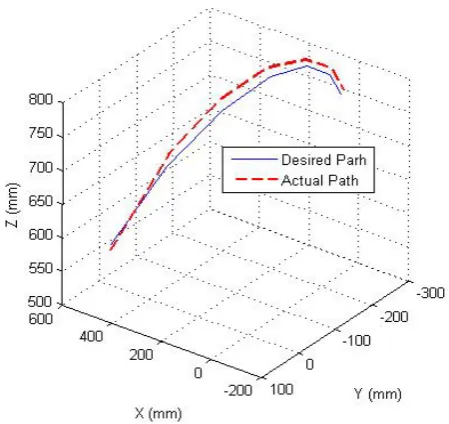
In order to obtain path accuracy of the 6R robot, a command path which consists of 7 command points is considered. The end-effector position is measured at these points by means of joint’s angular position measuring which is done by rotational potentiometers in each joint. Figure 10 shows the comparative diagrams of real and command angular position of the robot joints. Difference between command and actual position of the robot’s end-effector is shown in

Figures 11 and 12. Figure 11 shows the position of the end-effector on X, Y and Z axis and also 3D position of it, is shown in Figure 12. As a result, according to the Equation 36, path accuracy of this 6R robot is 13.3 mm [20-21].

6. CONCLUSIONS

(a) (b) (c)

Figure 9. The end-effectors' trajectory (a) Error on X axis, (b) Error on Y axis and (c) Error on Z axis.

-70 -60 -50 -40 -30 -20 -10 0

1 2 3 4 5 6 7

Target Points

A

n

g

u

la

r

P

o

si

ti

on

of

t

h

e 1st

J

o

in

t (d

e

g

) Actual Rotation(deg)

Desired Rotation(deg)

-35 -30 -25 -20 -15 -10 -5 0

1 2 3 4 5 6 7

Target Points

An

gu

la

r

Po

si

o

ti

o

n of

t

h

e

2

n

d

J

o

in

t. (d

e

g

)

Actual Rotation(deg) Desired Rotation(deg)

-80 -70 -60 -50 -40 -30 -20 -10 0

1 2 3 4 5 6 7

Target Points.

A

ngul

ar

P

o

s

iot

ion

of

t

he

4t

h

Jo

in

t.

(

d

e

g

)

Actual Rotation(deg) Desired Rotation(deg)

-65 -55 -45 -35 -25 -15

-5 1 2 3 4 5 6 7

Target Points

A

n

g

u

la

r P

o

si

ti

o

n

of

t

h

e

5t

h

Joi

n

t

(d

eg

)

Actual Rotation(deg) Desired Rotation(deg)

Figure 10. Command and measured angular motions.

procedure and performance testing of the 6R robot were developed. Verification of kinematics and dynamics of the robot was done by means of mathematical and computational modeling and simulation, using Mathematica, MATLAB and ADAMS software. Manufacturing and assembling procedure of the all mechanical parts of the robot were explained. The error of pose/path accuracy

-350 -150 50 250 450 650

1 2 3 4 5 6 7

Target Points

Com

m

an

d

and

re

al p

o

s

itio

n

of

th

e r

o

b

o

t’

s

e

n

d

-ef

fe

cto

r.(

mm)

X desired Y desired Z desired X Actual Y Actual Z Actual

Figure 11. Command and measured end-effectors' position on

X, Y and Z axis.

Figure 12. Command and measured end-effectors' 3D

position.

7. REFERENCES

1. Ahmadi, M., and Tamaddonkhah, A., “Design and Manufacturing a 3 Degree of Freedom Robot”, M.Sc. Thesis, Amirkabir University of Technology, Tehran, Iran, (1990).

2. Sattari, S., “Design and Manufacturing of Three Degree Robot”, M.Sc. Thesis, Sharif University of Technology, Tehran, Iran, (1999).

3. Mokhtari, M. H., “Manufacturing an Assembler Robot”,

M.Sc. Thesis, Iran University of Science and Technology, Tehran, Iran, (2000).

4. Liu, G., Iagnemma, K., Dubowsky, S. and Morel, G., “A Base Force/Torque Sensor Approach to Robot Manipulator Inertial Parameter Estimation”, IEEE International Conference on Robotics and Automation,

(1998).

5. Taylan, M., Das, L. and Canan Du, L., “Mathematical Modelling, Simulation and Experimental Verification of a Scara Robot”, Simulation Modelling Practice and Theory, Vol. 13, (2005), 257-271.

6. Maur cio, J., Mottaa, S. T., Guilherme, C. and Master, R. S., “Robot Calibration Using a 3D Vision-Based Measurement System with a Single Camera”,

Simulation Practice and Theory, Vol. 9, (2002),

293-319.

7. Miro, J. V. and White, A. S., “Modelling an Industrial Manipulator a Case Study”, Simulation Practice and Theory, Vol. 9, No. 6, (2002), 293-319.

8. Rosheim, M. E., “Robot Wrist Actuators”, Robotics Age, (1982), 15-22.

9. Rosheim, M. E. “A New pitch-Jaw-Roll Mechanical Robot Wrist Actuator”, Proc. of Robotics Conference SME, Vol. 15, No. 42, (1985), 20-15.

10. Colimitra, T., “Hand Gear Train”, U. S. Patent, 4, 683, 772, (1987).

11. Kung, C., “Spherical Robotic Shoulder Joint”, U. S. Patent, 5, 533, 418, (1996).

12. Rauchfuss, J. W., “Robotic Wrist Mechanism”, U. S. Patent, 6, 003, 400, (2000).

13. Wiitala, J. M., “Design of an Over Constrained and Dexterous Spherical Wrist”, Journal of Mechanical Design, Vol. 122, (2000), 347-353.

14. Hart, A. J., “Kinematic Coupling Interchange ability”,

Precision Engineering, Vol. 28, (2004), 1-15.

15. Schilling, R. J., “Fundamentals of Robotics Analysis and Control”, Prentice Hall, (1990).

16. Korayem, M. H., Jaafari, N., Jamali, Y. and Kiomarsi, M., “Design, Manufacture and Experimental Analysis of 3R Robotic Manipulator”, Paper in TICME, Tarbiat

Modares University, Tehran, Iran, (2005).

17. Korayem, M. H., Jamali, Y., Jaafari, N., Sohrabi, A. M. and Kiomarsi, M., “Design and Manufacturing a Robot Wrist: Performance Analysis”, Paper in TICME,

Tarbiat Modares University, Tehran, Iran, (2005). 18. “ISO 9283 Manipulating Industrial Robots Performance

Criteria and Related Test Methods”, International Standards Organization, (1998).

19. Abderrahim, M., “Kinematic Model Identification of Industrial Manipulators”, Robotics and Computer Integrated Manufacturing, Vol. 16, (2000), 1-8.

20. Korayem, M. H., Shiehbeiki, N. and Khanali, T., “Design, Manufacturing and Experimental Tests of Prismatic Robot for Assembly Line”, International Journal of AMT, Vol. 29, No. 3-4, (2006), 379-388.

21. Korayem, M. H., Shiehbeiki, N., “Performing Laboratory Tests for 3P Robot Using Vision”, 3rd IFAC Symposium on Mechatronic Systems, (September