Simulation of Gravity Wave Propagation in Free Surface Flows by an Incompressible SPH Algorithm

Simulation of Gravity Wave Propagation in Free Surface Flows by an Incompressible

SPH Algorithm

N. Amanifard *a_{, S. M. Mahnama}b_{, S. A. L. Neshaei} c_{, M. A. Mehrdad}c_{,M. H. Farahani}a

a_{Mechanical Engineering Department, University of Guilan, P.O. Box 3756, Rasht, Iran} b_{Islamic Azad University, Ramsar Branch, P.O. Box 465, Ramsar, Iran}

c_{Civil Engineering Department, University of Guilan, P.O. Box 3756, Rasht, Iran}

A R T I C L E I N F O

Article history:

Received 11September2008

Received in revised form 8 April 2011

Accepted 19April2012

Keywords:

Smoothed Particle Hydrodynamics (SPH) Lagrangian Method

Wave Propagation Free Surface

A B S T R A C T

This paper presents an incompressible smoothed particle hydrodynamics (SPH) model to simulate wave propagation in a free surface flow. The Navier-Stokes equations are solved in a Lagrangian framework using a three-step fractional method. In the first step, a temporary velocity field is provided according to the relevant body forces. This velocity field is renewed in the second step to include the viscosity effects. A Poisson equation is employed in the third step as an alternative for the equation of state in order to evaluate pressure. This Poisson equation considers a trade-off between density and pressure which is utilized in the third step to impose the incompressibility effect. The computations are compared with the experimental as well as numerical data and a good agreement is observed. In order to validate proposed algorithm, a dam-break problem is solved as a benchmark solution and the computational results are compared with the previous numerical ones.

doi:10.5829/idosi.ije.2012.25.03a.06

NOMENCLATURE

V particle velocity q=r/h non-dimensional distance between particles

V* particle first temporary velocity A a field variable

V** particle second temporary velocity B a vector

Vˆ particle corrected velocity without using XSPH D shear strain rate

V particle velocity by using XSPH correction T period of signals

P particle pressure Greek letters

t time  density of water

g gravitational acceleration * a temporary density

r position vector 0 initial density

x horizontal coordinate



shear stress tensor

y vertical coordinate  a scalar or vector quantity

W interpolation kernel  small number to avoid singularity

h smoothing distance  constant viscosity of water

m particle mass



constant XSPH correction

1. INTRODUCTION1

The study of wave propagation in free surface flows has many benefits and is being given great attention in

*_{Corresponding Author Email:[email protected] (N.}

Amanifard)

practice. Surface water waves have a high potential to cause damages and losses of lives in coastal areas. Predicting the damage of these waves is of importance when assessing risk and magnitude of flooding in these areas.

Previous investigations have been focused on the studies of wave propagation and overtopping through

Intrnational Journal of Engineering

using the experimental, analytical and numerical approaches. For example, Cox and Ortega [1] carried out an experimental study on the wave overtopping over a fixed deck using irregular and transient waves.

Unfortunately, due to the complexity of this phenomenon, number of reliable laboratory and field data is limited. Therefore, numerical methods are widely used for simulating of wave propagation.

Most of the numerical works on the recent wave problems have been carried out using the Eulerian grid-based methods with quite satisfactory results, such as finite element, finite volume and finite difference methods. These methods have provided many useful and satisfactory results. However, their successes largely rely on good quality meshes. The construction of such high quality mesh configurations is usually a difficult and time-consuming task, since it must be ensured that the aspect ratios of all elements are neither very large nor very small and thus the connectivity between nodes and elements must be carefully and accurately found and recorded. In addition, elements can frequently become over-distorted during the simulation of water wave evolutions. The over-distorted elements may be amended by remeshing. However, remeshing can be as expensive as the generation of original meshes and may take a major proportion of computational costs considering when this has to be done almost every time step.

A new class of methods has recently been developed, which can overcome the problems associated with mesh-based methods. These methods do not need using any mesh to discrete computational domains and they are only based on randomly-ordered and –distributed nodes. Many meshless (or particle) methods have been reported in the literature, such as meshless local Petrove–Galerkin (MLPG) method [2], moving particle semi-implicit (MPS) method [3], smoothed particle hydrodynamics method (SPH) [4] and so on. Among them, the SPH method has been used widely to simulate water wave problems [4-6].

The SPH method uses a purely Lagrangian approach and has been successfully employed in a wide range of applications, such as incompressible fluid flow, multiphase flow, turbulence, heat and mass transfer, elasticity and fracture, and etc [7]. Recently, SPH has also been employed to simulate fluid-structure interaction [8-10]. The meshless characteristic of SPH makes the method needless of using data connectivity as needed by the finite volume and finite element methods. This gives the method a very useful feature when dealing with complex flows exhibiting large deformations and/or free-surfaces.

The method was originally developed by Lucy [11] and Gingold and Monaghan [12] to solve compressible astrophysical problems, and then it was later extended to incompressible flows by Monaghan [4]. Several other

researchers have contributed to the method and solved various engineering problems including turbulent flows, interfacial flows and sloshing problems [13-15].

Dalrymple et al. [5] and Gomez-Gesteira et al. [16] employed this method to study the wave overtopping over coastal structures. In the previous simulations of incompressible flows using the SPH model, the incompressibility was achieved by employing an equation of state and the fluid was assumed to be slightly compressible. This approach is denoted as the weakly compressible SPH, since a large enough sound speed has to be introduced into the pressure equation to ensure the numerical stability. Based on the semi-implicit algorithm of the MPS method [3], a truly incompressible version of the SPH [17] has been proposed, in which the free surfaces were identified and tracked by particles without numerical diffusion. The key difference between the original weakly compressible SPH [11, 12] and the incompressible SPH [17] lies in that the former calculates the pressure using an equation of state, while the latter employs a strictly incompressible SPH formulation, in which the pressure is not an explicit thermodynamic variable but obtained implicitly through solving a pressure Poisson equation derived from the mass and momentum equations. In this sense, it is also very similar to the pressure projection method widely used in grid based methods and the projection SPH of Cummins and Rudman [18].

In this paper a new incompressible SPH algorithm based on Shaoet al.[17] is presented to simulate gravity wave propagation in free surface flow problems. Before this simulation, in order to show the ability of the method for simulating of free surface problems, a dam-break problem is modeled as a benchmark and the results are compared with the results of standard SPH method.

The proposed algorithm is similar to three step explicit SPH algorithm proposed by Hosseini et al. [19] for simulation of incompressible fluid flows. In the first step of this algorithm, the momentum equation is solved in the presence of the body force neglecting all other forces. The calculated temporary velocities are renewed in the second step to include the viscosity effect. A Poisson equation is employed in the third step as an alternative of the equation of state in order to evaluate pressure of the particles. This Poisson equation considers a trade-off between density and pressure which is utilized in the third step to impose the incompressibility effect.

even successfully applied to other fluid problems, is usually required to be carefully refined when it is applied to water waves. The SPH computations are compared with the experimental data of Cox and Ortega [1] and the numerical results of Gomez-Gesteira et al. [16].

2. GOVERNING EQUATIONS

The governing equations for simulating free surface flow in 2-D dimensions are the mass and momentum conservation equations. With regard to fluid particles, they are written in Lagrangian form as:

1 . 0 D V Dt 

    (1)

1 1

.

DV

P g

Dt   



      (2)

Equation (1) is in the form of a compressible flow. The purpose is that the deviation of fluid densities at the particle can then be used to enforce incompressibility in the correction step of time integration.

3. SPH FORMULATION

The SPH formulations as developed by Monaghan [20] are obtained by interpolating from a set of points that may be disordered. The interpolation is based on the theory of integral interpolants using kernels that approximate a delta function. The interpolants are analytic functions that can be differentiated without the use of grids. If the points are fixed in position, the equations reduce to finite difference equations, with different forms depending on the interpolation kernel. The SPH equations describe the motion of the interpolating points, which can be assumed as particles. Each particle carries a mass m, a velocity

V

, and other properties, depending on the problem.

3. 1. Interpolation Using the above concepts, any quantity of particle i, whether scalar or vector, can be

approximated by the direct summation of the relevant quantities of its neighboring particles j

 

 

_{ }

W



r r h



r r m

r i j

j j j j j j i

i 



_  ,



 (3)

where iand j= reference particle and its neighbors.

3. 2. Kernel The use of different kernels is the SPH analogue of using different schemes in finite difference methods. While different equations can have different kernels, usually the same kernel is used throughout all formulations in one model. By balancing the

computational accuracy and efficiency, the following kernel based on the spline function and normalized in 2-D is adopted [20]

 





2 3 3 2 3 3 1 1 2 4 10 1

, 2 1 2

7 4

0 2

q q q

W r h q q

h q   _{ }  _    _{ }                     (4)

The smoothing distance or kernel range hdetermines

the degree which a particle interacts with neighboring particles.

This kernel has the advantage of possessing compact support, the second derivative being continuous and the dominant error term in the integral interpolant being the order of h2. The continuity of the second derivative

means that the kernel is not too sensitive to particle disorder and the errors in approximating the integral interpolants by summation interpolants are small provided the particle disorder is not too large.

3. 3. Gradient, Divergence and Laplacian The formulation of the gradient term in the Navier–Stokes equation has different forms depending on the derivation used [20]. The following symmetric forms are employed for gradient of a scalar Aand divergence

of a vector Bsince it conserves linear and angular momentum exactly ij i j j i i j j i i W A A m

A _

       





_{2 2}

1    (5) ij i j j i i j j i i i W B B m

B _

        .



. 1 2 2 _   (6)

where the summation is over all particles other than particle i and iWij  gradient of the kernel taken with respect to the positions of particle i. In practice

only near neighbors contribute, because the kernel has a finite range.

A simple way to formulate the Laplacian operator is to envisage it as dot product of the divergence and gradient operators. This approach proved to be problematic as the resulting second derivative of the kernel is very sensitive to particle disorder and when dealing with the Navier-Stokes equations can easily lead to pressure instability and decoupling in the computation due to the co-location of the velocity and pressure. In this paper, the following alternative approach is adopted [17]





2 2 2

. 8 1 .                



ij ij i ij ij j i j j i r W r A m A ₍₇₎

where A_ij A_iA_j,r_ij r_ir_j and  is a small

4.THREE-STEP INCOMPRESSIBLE SPH ALGORITHM

In this section, an algorithm is presented to show the sequence of computation of each term in the governing equations. In this paper, a fully explicit three-step algorithm is used. In the first step of this algorithm, the momentum equation is solved in the presence of the body forces neglecting all other forces. As a result, an intermediate velocity is computed as

t g V

V*  _t   (8)

Our experience has shown that it is important to impose the body forces in the first step of the solution algorithm especially in highly viscous fluids. In the second step, the calculated intermediate velocities are employed to compute the divergence of the stress tensor. Generally speaking, viscosity of incompressible generalized Newtonian fluids depends only on the second principal invariant of the shear strain

rate ( T)/2

V V

D   , i.e.,



 j i ij ijD D D , (9)

A classical constitutive law for these generalized Newtonian fluids is given by

 

D D 

  (10)

For Newtonian fluids the familiar form   2D is

recovered.

Consequently, the stress tensor

 

 can be calculated for any specified constitutive law. In this work, the divergence of the stress tensor in the momentum equation is obtained as:

 

r h W

m i ij

j j j i i j i , . .                  _

_

  2 2 1       (11)

At the end of second step, the velocity components of each particle is updated according to:

t V

V _

     _     . * * * 1 (12)

At this stage, each particle is moved according to its second intermediate velocity **



**_, **



v u

V  .

Thus far no constraint has been imposed to satisfy the incompressibility of the fluid and it is expected that the density of some particles change during this updating. In fact, with the help of the continuity equation one can calculate the temporal fluid density of each particle as:



V V



W

 

r h m Dt D ij i j j i j

i 



 _. _, 

(13)

The velocity field



V

 

u,v



which is needed to

restore the density of particles to their original values is now calculated. To do this, in the third step of the

algorithm, the momentum equation with the pressure gradient term as a source term is combined with the continuity Equation (1) as

0 . 1 * 0 0      V t     (14) t P

V _

     _   1_*





(15)

to obtain the following pressure Poisson equation

2 0 * 0 * 1 . t P          _      (16)

Equation (16) can be discretized according to Equation (7) to obtain the pressure of each particle as:









* 0

2 _* 2 2 ₂

0

1

2 2 ₂

*

8 .

8 .

j j ij i ij i

i

j i j ij

j ij i ij

j i j ij

m P r W

P

t _r

m r W

r    _{  }                                 





(17)

Using Equation (17) for the pressure of each particle, one can calculate V according to Equations

(15) and (5) as

ij i j j j i i j i W P P m t

V _

        





_*2 _2 



(18)

Finally, the velocity of each particle at the end of time-step will be obtained as:

V V

V_tt  **   ₍₁₉₎

and the final position of particles are calculated using a central difference scheme in time.



t t t



t t

t V V

t r

r     

2 (20)

This completes the computations required for one time-step. The procedure should be repeated for every other time-step till a desired time is reached

5. TREATMENT OF FREE SURFACE AND WALL BOUNDARY CONDITION

No special treatment was applied on free surface particles in the computational domain. In fact in this SPH method free surface is modeled naturally and this is one of the main advantages of the method.

mirror the physical properties of inner fluid particles, so that boundary conditions are strictly satisfied along the solid walls [18].

Here we follow the treatment used by Koshizuka et al. [22] to model the wall boundaries by fixed wall particles, which are spaced according to the initial configuration. The Poisson Equation (16) is solved on these wall particles to repulse the inner flow particles accumulating in the vicinity of the wall. In this sense, the wall particles are dependent on the inner flows. For example, the pressure of wall particles increases when the particle density in the vicinity of the wall increases and thus the inner fluid particles are repelled from the wall, and vice versa.

6. MODEL VERIFICATION

In order to validate of the present model, a dam-break problem is solved as a benchmark problem and the computational results are compared with other numerical works. A schematic of the dam break model is presented in Figure 1. In this model, the tank is

m

L3.22 long and H2.0m high. A column of water (L_w 1.2mandH_w 0.6m) is located in the left side of the tank.

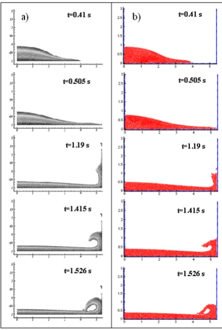
Figure 2 presents some snapshots of the flow at different times. The computed results are compared with the numerical results in which the standard SPH method is used to simulate the global development of fluid flow in dam-break problem [14].

At time t = 0s (not shown in the figure) the water column is allowed to flow. A relatively high velocity and shallow water depth flow in the xdirection quickly

forms (e.g. t = 1.19s). As time progresses, the flow impacts on the vertical wall at the opposite side of the tank. An upward water jet is suddenly formed that rises until gravity overcomes the upward momentum (around t = 1.19s). At this moment, the jet becomes thicker and the flow starts to reverse. Due to the oncoming flow, an adverse momentum gradient is created that results in an overturning wave (around t = 1.415s). This wave formation continues until the wave tip reconnects with the incident shallow water flow that now has less forward momentum. (Before t = 1.526s).

Figure 1.General layout of dam-break problem

Figure 2.Dam-break flow and impact against a vertical wall. a) Calculation by using standard SPH [14] b) Simulation by present incompressible SPH method

A good agreement in free surface shapes is observed by comparing between the results of standard SPH and present incompressible SPH method.

7. THE WAVE PROPAGATION PROBLEM

In this section, the presented incompressible SPH model is employed for simulating waves generated by a wave-maker to reproduce the experimental data and previous numerical results.

the far wall. The free surface positions were measured to cover the area of interest in the experiment.

7. 2. Computational Parameters Following the experimental setting of Cox and Ortega [1], the numerical tank is taken to be 17.3 m long and 1.2 m high. The length of numerical tank is shorter than the experimental one due to the constraint of the CPU time. The initial water depth is 0.65 m. The numerical wave tank used in this paper is shown in Figure 3.

The incident wave is generated by moving a numerical wave paddle located at the offshore boundary. The numerical wave signals are similar to those used by Gomez-Gesteira et al. [16].

Figure 3.Numerical wave tank

Figure 4.Particle configurations during wave propagation

computed by the present method at different times.

7. 3. Discussion of Results In this section, particle configuration due to the movement of the wavemaker is presented in Figure 4 at different times. In this computation, fluid particles are initially placed on a regular and equally spaced Cartesian grid with dx = dy = 0.04 m and thus approximately 9000 particles are used in the simulation. This number of particles ensures the accuracy of computations with respect to reduce the CPU time. A constant time step (dt = 0.00001s) and an initial particle velocity and pressure (V = P = 0) are used in the computations. The main computations using these quantities can be finished within 6 hours by a CPU 1.87GHz and RAM 1.0GB PC.

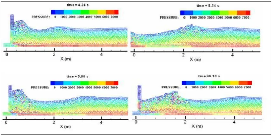
Figure 6.Pressure field of fluid during wave propagation at different times

The generated waves move toward the right wall corresponding to the wavemaker movement. The figure illustrates the stability of the present method to simulate the problems for long times.

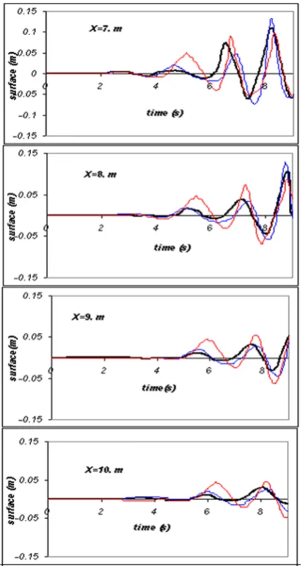
In order to compare our results to the experimental ones [1] and numerical results in which the weakly compressible SPH is used to simulate propagation of waves in the tank [16], the numerical free surface position at different times is shown in Figure 5. The four frames correspond to the different positions from x=7.0 to 10.0 m, measured from the wavemaker. The numerical signal is observed to be in good agreement with the experimental one, both in phase and amplitude, although there are several slight discrepanciesbetween theexperimental and numerical profiles.

This is probably due to the fact that the numerical signal was filtered using a low pass filter, in such a way that sharp peaks are considerably smoothed out. Moreover, it is evident that the results provided by the current presented SPH algorithm shows more compatible results with experiments than those reported by weakly compressible SPH [16] especially in the case of amplitude.

It is noteworthy that in the previous simulations using weakly compressible SPH a tendency to form clump has been reported. However, investigation of Hosseini et al. [8] illustrates that the three step SPH algorithm shows no tendency to particle clustering. Although this numerical instability is insignificant in fluid simulations, it can result in an artificial surface tension. This characteristic prevents forming high

curvature regions because of large density discontinuities.

In Figure 6 the computed pressure field at different times is presented. These pressure contours show that the pressure of free surface particles is about zero and grows gradually with increase in water depth, hence the maximum pressure of fluid (about 7000 pa) belongs to the beneath particles.

8. CONCLUSION

9. REFERENCES

1. Cox, D.T. and Ortega, J.A., “Laboratory observations of green water overtopping a fixed deck”, Ocean Engineering, Vol. 29, (2002), 1827–1840.

2. Ma, Q.W., “Meshless local Petrov–Galerkin method for two-dimensional nonlinear water wave problems”, Computational Physics, Vol. 205, (2005), 611–625.

3. Koshizuka, S., Tamako, H. and Oka, Y., “A particle method for incompressible viscous flow with fluid fragmentation”, Computational Fluid Dynamics,Vol. 4, No. 1, (1995), 29–46. 4. Monaghan, J.J., “Simulating free surface flows with SPH”,

Computational Physics,Vol. 110, (1994), 399–406.

5. Dalrymple, R.A. and Rogers, B.D., “Numerical modeling of water waves with the SPH method”, Coastal engineering,Vol. 53, (2006), 141-147.

6. Lo E.Y.M. and Shao S.D., “Simulation of near-shore solitary wave mechanics by an incompressible SPH method”, Applied Ocean Research,Vol. 24 (5), (2002), 275–286.

7. Monaghan J.J., Smoothed particle hydrodynamics. Reports on Progress in Physics, Vol. 68, (2005), 1703–1759.

8. Hosseini, S. M. and Amanifard, N., “Presenting a modified SPH algorithm for numerical studies of fluid-structure interaction problems”, International Journal of Engineering. Transactions B: Applications,Vol. 20, (2007), 167-178. 9. Farahani, M.H., Amanifard, N. and Pouryoussefi, Gh., 2008.

“Numerical simulation of a pulsatory flow moving through flexible walls using smoothed particle hydrodynamics”, Proceeding of Int. Conference of Mechanical Engineering (ICME 2008), 2008 World Congress of Engineering, London, UK, pp 1337-1341, July, 2008.

10. Farahani, M.H., Amanifard, N., Asadi, H. and Mahnama, M., “Fluid structure interaction simulation with free surface flows by smoothed particle hydrodynamics”, ASME Int. Mechanical Engineering Congress & Exposition, Technical Publication (IMECE2008-66769) Boston, Massachusetts, USA, 2008. 11. Lucy, L. B., A numerical approach to the testing of the fission

hypothesis.Astronomical Journal,Vol. 82, (1977), 1013–24.

12. Gingold, R. A. and Monaghan, J. J., “Smoothed particle hydrodynamics: theory and application to non-spherical stars”, Monthly Notices of the Royal Astronomical Society,Vol. 181, (1977), 375–89.

13. Welton W., “Two-dimensional PDF/SPH simulations of compressible turbulent flows”, Computational Physics, Vol. 139,(1998), 410–443

14. Colagrossi A. and Landrini M., “Numerical simulation of interfacial flows by smoothed particle hydrodynamics”, Computational Physics, Vol. 191, (2003), 448–475

15. Kelecy F.J. and Pletcher R.H., “The development of a free surface capturing approach for multidimensional free surface flow in closed container”, Computational Physics, Vol. 138, (1997), 939-980.

16. Gomez-Gesteira, M., Cerqueiro, D., Crespo, C. and Dalrymple, R.A., “Green water overtopping analyzed with a SPH model”, Ocean Engineering, Vol. 32, (2005), 223–238.

17. Shao, S. and Lo E. Y. M., “Incompressible SPH method for simulating Newtonian and non-Newtonian flows with a free surface”, Advances in Water Resources,Vol. 26, (2003), 787‒

800.

18. Cummins, S. J. and Rudman, M., “An SPH projection method”, Computational Physics,Vol. 152, (1999), 584 607.

19. Hosseini, S. M., Manzari, M. T. and Hannani, S. K., “A fully explicit three step SPH algorithm for simulation of non-Newtonian fluid flow”, International Journal of Numerical Methods for Heat&Fluid Flow,Vol. 17, (2007), 715–735.

20. Monaghan J. J., “Smoothed particle hydrodynamics”, Annual Review of Astronomy and Astrophysics,Vol. 30, (1992), 543– 74.

21. Monaghan J.J. and Kos A., “Solitary waves on a Cretan beach”, Wtrwy, Port, Coastal and Ocean Eng., Vol. 125(3), (1999), 145–154.

Simulation of Gravity Wave Propagation in Free Surface Flows by an Incompressible

SPH Algorithm

N. Amanifarda_{, S. M. Mahnama}b_{, S. A. L. Neshaei} c_{, M. A. Mehrdad}c_{,M. H. Farahani}a

a_{Mechanical Engineering Department, University of Guilan, P.O. Box 3756, Rasht, Iran} b_{Islamic Azad University, Ramsar Branch, P.O. Box 465, Ramsar, Iran}

c_{Civil Engineering Department, University of Guilan, P.O. Box 3756, Rasht, Iran}

A R T I C L E I N F O

Article history:

Received 11September2008

Received in revised form 8 April 2011

Accepted 19April2012

Keywords:

Smoothed Particle Hydrodynamics (SPH) Lagrangian Method

Wave Propagation Free Surface

هﺪﯿﮑﭼ

ﻢﮐاﺮﺗ لﺪﻣ ﮏﯾ ،ﻪﻟﺎﻘﻣ ﻦﯾا راﻮﻤﻫ تارذ ﮏﯿﻣﺎﻨﯾدورﺪﯿﻫ ﺮﯾﺬﭘﺎﻧ

) SPH ( ﻪﯿﺒﺷ ياﺮﺑ ار دازآ ﺢﻄﺳ نﺎﯾﺮﺟ رد جﻮﻣ رﺎﺸﺘﻧا يزﺎﺳ

ﯽﻣ ﻪﺋارا ﺪﻫد . ﺮﯾوﺎﻧ تﻻدﺎﻌﻣ

-ﻪﺑ ،ﺲﮐﻮﺘﺳا ﻪﻠﺣﺮﻣ ﻪﺳ ﻢﺘﯾرﻮﮕﻟا ﮏﯾ زا هدﺎﻔﺘﺳا ﺎﺑ يﮋﻧاﺮﮔﻻ ترﻮﺻ ﯽﻣ ﻞﺣ يا

ﺪﻧﻮﺷ . مﺎﮔ رد

ﺑ ﯽﻧﺎﯿﻣ ﺖﻋﺮﺳ ناﺪﯿﻣ ﮏﯾ ،ﯽﻤﺠﺣ يﺎﻫوﺮﯿﻧ زا هدﺎﻔﺘﺳا ﺎﺑ ،لوا ﻪ

ﯽﻣ ﺖﺳد ﺪﯾآ . تاﺮﺛا لﺎﻤﻋا ﺎﺑ ،مود مﺎﮔ رد ﺖﻋﺮﺳ ناﺪﯿﻣ ﻦﯾا

ﯽﻣ ﺪﯾﺪﺠﺗ ،ﺖﺟﺰﻟ دﻮﺷ

. ﻪﺑ نﻮﺳاﻮﭘ ﻪﻟدﺎﻌﻣ ﮏﯾ ،مﻮﺳ مﺎﮔ رد ﻪﺑ رﺎﺸﻓ ﻪﺒﺳﺎﺤﻣ ياﺮﺑ ﺖﻟﺎﺣ ﻪﻟدﺎﻌﻣ ﻦﯾﺰﮕﯾﺎﺟ ناﻮﻨﻋ

رﺎﮐ ﻪﺘﻓﺮﮔ

ﯽﻣ دﻮﺷ . ﻪﻧزاﻮﻣ ،نﻮﺳاﻮﭘ ﻪﻟدﺎﻌﻣ ﻦﯾا ار يا

ﯽﻣ دﺎﺠﯾا رﺎﺸﻓ و ﯽﻟﺎﮕﭼ ﻦﯿﺑ ﻢﮐاﺮﺗ لﺎﻤﻋا ياﺮﺑ مﻮﺳ مﺎﮔ رد نآ زا ﻪﮐ ﺪﻨﮐ

يﺮﯾﺬﭘﺎﻧ

ﯽﻣ هدﺎﻔﺘﺳا دﻮﺷ . ﺖﺳا هﺪﺷ هﺪﻫﺎﺸﻣ ﯽﺑﻮﺧ ﻖﻓاﻮﺗ و هﺪﺷ ﻪﺴﯾﺎﻘﻣ ﺮﮕﯾد ﯽﻫﺎﮕﺸﯾﺎﻣزآ و يدﺪﻋ ﺞﯾﺎﺘﻧ ﺎﺑ تﺎﺒﺳﺎﺤﻣ ﺞﯾﺎﺘﻧ .

ﻪﺑ ﻪﺑ ،ﺪﺳ نﺪﺷ ﻪﺘﺴﮑﺷ ﻪﻟﺄﺴﻣ ،هﺪﺷ ﻪﺋارا شور ﺖﺤﺻ ﯽﺳرﺮﺑ رﻮﻈﻨﻣ ﻪﯾﺎﭘ ﻪﻟﺄﺴﻣ ﮏﯾ ناﻮﻨﻋ

ا ﺑ ﺞﯾﺎﺘﻧ و هﺪﺷ ﻞﺣ ي ﻪ

هﺪﻣآ ﺖﺳد

شور زا ﻞﺻﺎﺣ ﺞﯾﺎﺘﻧ ﺎﺑ ﺖﺳا هﺪﺷ ﻪﺴﯾﺎﻘﻣ ﺮﮕﯾد يدﺪﻋ يﺎﻫ

.