TECHNICAL NOTE
THE ANALYSIS OF LONGITUDINAL SHRINKAGE IN BUTT
WELD JOINT
M. Iranmanesh* and S. Babakoohi
Department of Marine Engineering, Amirkabir University of Technology P. O. Box 15875-4431, Tehran, Iran
[email protected] - [email protected]
*Corresponding Author
(Received: December 2, 2006 - Accepted in Revised Form: January 30, 2008)
Abstract In this research longitudinal shrinkage of two steel plates with identical thickness that are joint together through butt welding and another steel plate with bead welding. This study begins with the introduction of a model, in which the thermoelastoplastic zones near the weld line is simulated with a thermoelastoplastic flat bar, and full-elastic areas beyond the weld line is simulated with a full elastic springs, by proposing the physical terms of the model and favorite presumptions, the related equations are solved and eventually the conclusion is a relation which can be used to calculate the amount of longitudinal shrinkage with acceptable accuracy.
Keywords Butt Weld Joint, Distortion, Longitudinal Shrinkage, Thermoelastoplastic
ﻩﺪﻴﻜﭼ
ﺖﻣﺎﺨﺿﺎﺑﯼﺩﻻﻮﻓﻕﺭﻭﻭﺩﺭﺩﯽﻟﻮﻃﺽﺎﺒﻘﻧﺍ،ﻖﻴﻘﺤﺗﻦﻳﺍﺭﺩ ﻳ
ﺐﻟﻪﺑﺐﻟﺵﻮﺟﻪﻄﺳﺍﻭﻪﺑﻪﮐﻥﺎﺴﮑ
ﻞﺼﺘﻣ ﺮﮕﻳﺪﮑﻳ ﻪﺑ ﺖﺳﺍ ﻪﺘﻓﺮﮔ ﺭﺍﺮﻗ ﯽﺳﺭﺮﺑ ﺩﺭﻮﻣ،ﺪﻧﺍ ﻩﺪﺷ
. ﯽﺣﺍﻮﻧ ﻥﺁﺭﺩ ﻪﮐ ﻩﺪﺷ ﻒﻳﺮﻌﺗ ﯽﻟﺪﻣ ﺭﻮﻈﻨﻣﻦﻳﺪﺑ
ﻮﺘﺳﻻﺍﻮﻣﺮﺗ ﻪﻤﺴﺗ ﮏﻳﺎﺑﺵﻮﺟ ﻂﺧﮏﻳﺩﺰﻧﮏﻴﺘﺳﻼﭘ
ﻂﺧﺯﺍﺮﺗﺍﺮﻓﮏﻴﺘﺳﻻﺍﻡﺎﻤﺗﯽﺣﺍﻮﻧﻭﮏﻴﺘﺳﻼﭘﻮﺘﺳﻻﺍﻮﻣﺮﺗ
ﻭﻩﺪﺷﯼﺯﺎﺳﻪﻴﺒﺷﮏﻴﺘﺳﻻﺍﻡﺎﻤﺗﺮﻨﻓﻭﺩﺎﺑﺵﻮﺟ ﺕﺎﺿﻭﺮﻔﻣﻭﻝﺪﻣﺮﺑﻢﮐﺎﺣﯽﮑﻳﺰﻴﻓﻂﻳﺍﺮﺷﻒﻳﺮﻌﺗﺎﺑ
ﺮﻈﻧﺩﺭﻮﻣ
ﯽﺒﺳﺎﻨﻣ ﺖﻗﺩ ﺎﺑ ﺍﺭ ﯽﻟﻮﻃ ﺽﺎﺒﻘﻧﺍ ﺭﺍﺪﻘﻣ ﻥﺁ ﮏﻤﮐ ﻪﺑ ﻥﺍﻮﺗ ﯽﻣﻪﮐ ﺪﻳﺁ ﯽﻣ ﺖﺳﺪﺑ ﯼﺍ ﻪﻄﺑﺍﺭ ،ﺕﻻﺩﺎﻌﻣ ﻞﺣ ﻭ ﺩﻮﻤﻧﻪﺒﺳﺎﺤﻣ .
1. INTRODUCTION
In welding process, the heating and cooling cycle causes shrinkage in both base and weld metal and subsequently shrinkage tend to cause distortion in members and/or metal structures. The word distortion means unconventional deformation in the welded structure in several different form or combinedsuch as buckling, bending which results various dimentional changes in metal structures during and after the welding process that leads to disarrange connections and its removal sustains heavy costs.
Longitudinal shrinkage is one of the dimentional changes in parallel butt weld and bead weld joint. It is an important factor in welding
sheet metal, because this is the main factor for buckling along the weld line.
Researchers have studied dimentional changes as longitudinal shrinkage by analytical, numerical and finite element methods. The practical experimental methods which have been used for proving the correctness of theorical methods and/or methods themselves, wrote such empirical relations.
L
2B 2Lep
t
K
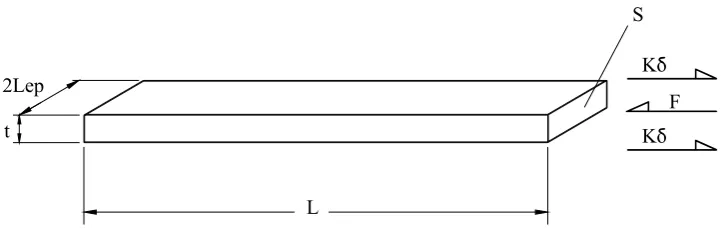
Figure 1. The model of longitudinal shrinkge process analysis.
Ko F 2Lep
t
L
Ko S
Figure 2. Balance of forces in model. movement process were studied finally on suitable
equation for calculating residual longitudinal shrinkage in a butt weld joint and in bead weld is introduced. Comparision of obtained quantities from this method and experimental samples are the other matters which have been studies in this paper.
2. DESCRIPTION OF MODEL AND ASSUMPTIONS
Debated model is shown in Figure 1, in which the thermoelastoplastic zone of two plates is simulated with a thermoelastoplastic flat bar which has 2Lep width, t thickness and L length and the rest of plates which have full elastic behavior are simulated with two full elastic spring with K equivalent spring constant.
In this model physical property is assumed constant; heat flow similar to bidimentional quasi-stationary state and in conforming with Equations 1 and 2, the yield
σy = σyo [1 - (T/Tm)] (1)
Ey = Eo [1 - (T/Tm)] (2)
σyo and Eo are yield stress and modulus of elasticity at room temperature respectively. Tm is melting temperature of metal.
3. ANALYSIS OF MODEL
In heating cycle, the thermoelastoplastic flat bar of model was expanded and resistance forces of springs contract the flat bar, thus, regarding to description of model, the elastic strain of flat bar is written as follows:
ε = δ/L = εe + αT (3)
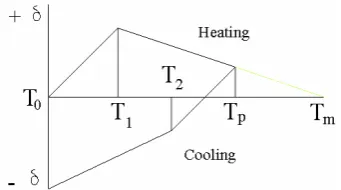
Figure 3. Diagram of displacement - temperature in model.
εe = σ/E (4)
according to Figure 2, F = - 2Kδ, (F is spring force), thus:
σ = F/S = - 2Kδ/S (5)
For easy calculation, dimentionless parameter Kr is defined as follows:
Kr = (spring constant divided by flat bar constant)
= (2K) / (EoS/L) (6)
S is cross section of model's flat bar, and is equal with; S = 2t Lep. with intersection of Equations 2,3,5 and 6 together and simpllify we have:
δ =[ (Tm-T) / [Tm (1+Kr ) -T] αTL (7)
Equation 7 gives the relationship between displacement of model’s flat bar and temperature before it attains the plastic state. When the temperature is higher than the yield temperature, the displacement is obtained from Equation 8 as follows:
σy = σyo (1-T/Tm) → Fy/S = (Fyo/S) (1-T/Tm)
(8)
Substituting F = - 2Kδ into Equations 8 and 5:
δ = + δyo(1-T/Tm) (9)
with substituting yield temperature T1 into Equations 7 and 9 and equalizing both obtainded δ
from both equations, we have:
T1 = [(Kr+1)σyoTm]/[α Tm Eo Kr + σyo] (10)
When heating the flat bar is finished, the flat bar enters cooling phase and during this stage, if there is no plastic deformation, the strain change will be as follow:
Δε = δ/L - δp/L = (σ/E+αT) – (σp/E+αTp) →δ
/L-δp/L = (σ/E-σp/E) + α(T-Tp) (11)
{p} index is the indicator of heating phase therefore Equation 9 can be used for calculating δp:
δp = δyo (1-Tp/Tm) (12)
if Equation 11 is substituted by Equations 2, 5 and 12, at last:
δp = δyo (1-Tp / Tm) - {[(Tm-T) (Tp-T)αL] /
[Tm(1+K)-T]} (13)
Equation 13 is reliable in temperatures between T2 and Tp (T2 ≤ T < Tp), and T2 is elastic to plastic deformation temperature used in cooling phase (Figure 3). During cooling phase, if tension force of springs leads the flat bar to plastic deformation, regarding Equation 9, the amount of displacement can be obtained from following equation:
δ = - δyo(1-T/Tm) (14)
The minimum of Kr for the purposes of producing plastic deformation in the flat bar during the heating phase can be resulted when T1 and Tp are of equal amount in relation (10), (T1 = Tp). In this way, Kr is named Krco or critical relative stiffness:
Krco= [σyo (Tm-Tp)] / [(αEoTp-σyo)Tm] (15)
In Equation 13, based on Figure 3, if T = 0, then the minimum Kr that causes plastic deformation in model flat bar during cooling phase equals:
Krc1 = [(2Tm – Tp) σyo] / [α TmTpEo – (2Tm –
Tp) σyo] (16)
several strips, the maximum temperature in each strip will be between Tm and Tc(Tm ≥ Tp ≥ Tc). Tm is steel melting temperature and Te is Lep boundry temperature in each plate which is 350˚C for mild steels [2]. Therefore Lep begins from center of weld line and extends up to the point which its maximum temperature is 350˚C. For calculating the Lep we can use the Adams’s maximum temperature equation [3] which has been resulted from Rosenthal's analytic equation [4]. This equation in bidimensional aspect is as following below:
1/(Tp-To) = (4.133 cρtvy) /(ηEpI) (17)
(cρ: Volumetric specific heat, v: Electrode speed, Ep and I: Welding voltage and Current)
Therefore if 350˚C is substitute for Tp, then y equals Lep as coming below:
Lep = [(ηEpI)/(4.133cρtv)] [1/(350˚C -To)] (18)
In any situation if we extract Krco and Krc1 from Equations 15 and 16 in temperature, Te = 350˚C and Tm, for a mild steel having average physical properties and constants, it will be as mentioned bellow:
Krco at 350˚C ≈ 0.3 / Krc1 at 350˚C ≈ 1 /Krco at Tm ˚C = 0 /Krc1 at Tm˚C ≈ 0.07 (19)
Kr can be calculated as below:
Kr = (2K)/(SEo/L) = [2(B-Lep)tEo/L]/[2LeptEo/L]
= (B-Lep)/Lep (20)
If Lep = 0.5B (In welding, actually, Lep is an insignificant fraction of B. thus Lep = o.5B is a inprobable assumption), then Kr = 1. Therefore referring to calculations (19) we can conclude that in heating and cooling phases, plastic deformation in the model's flat bar is observed and the residual shrinkage is calculated with substituting 0 instead of T in Equation 14:
δr = -δyo = - (σyo/Eo) (L/Kr) (21)
Therefore we can use Equation 21 if K ≥ 1. When K
is grater than 1, the accuracy of equation increases because the constructed model becomes closer and will have more resemblance to the real one. Figure 4 demonstrates a sample of bead weld [5] that has been tried under the conditions mentioned in Table 1. The results of the tests have been put in the same table as the one that shows, if K increases more than 1, the answer's accuracy increas.
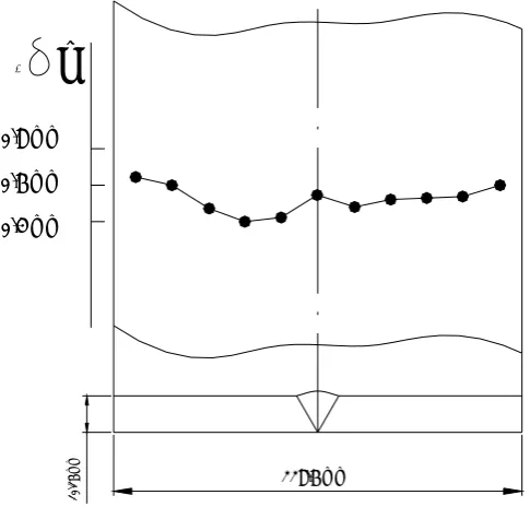
Figure 5 shows the distribution of residual longitudinal shrinkage in a sample [5] (in the form of absolute) is 0.515mm that in comparison with δr = 0.6 mm resulted from Equations 20 and 21 is indicator of an acceptable accuracy of equations produced by the model used in this analysis.
4. CONCLUSIONS
In this article, the principle of heat transfer theory has been built on the basis of Rosenthal's bidimentional heat flow theory. Therefore it is expected from the final results of this analysis to have relative and appropiate answer for plates possessing thickness of up to 10 mm. Lengthiness of welding line and the movement of welding electrode at a constant velocity are of the essence in quasistationary state heat flow. quasistationary state heat flow is one of the characteristics of Rosental's analysis, it is possible to use the final equation of this model for welding processes of plates with large dimensions involved in metal heavy industries including shipbuilding.
As shown in Figure 5, respecting this point that the distribution of longitudinal shrinkage doesn't appear to distribute evenly in the width of the plate the relation represented by this analysis at the end, calculates the average quantity of longitudinal shrinkage in the width of the plate (evenly) with satisfactory accuracy.
6. REFRENCES
1. Moshaiv, A. and Song, H., “Near and far Field Approximation for Analyzing Flame Heating and welding”, Journal of Thermal Stresses, Vol. 13,
(1990), 1-19.
914mm
305mm
6.35mm
Figure 4. Dimensions of bead weld sample.
TABLE 1. Parameters and Results in Sample of Weld Bead.
Sample I(A) Ep(V) V(mm/s) Lep(mm) Krc δr(mm)
Model
δr(mm) Sample 1 100 25 2.5 22.6 5.74 0.28 0.34 2 170 27 2.4 43.3 2.52 0.63 0.54
3 200 30 2.2 61.77 1.47 1 0.70
σyo = 350 Mpa, Eo = 200 Gpa, η = 0.85(Arc efficiency), cρ = 0.0044 j/mm ≤
0.8 mm
0.6 mm
0.4 mm
228.6 mm
10
.1
6
m
m
-
r
Figure 5. Longitudinal shrinkage distribution in the sample (butt welding)
3. Adams, M., “Cooling rates and Peak Temperatures”,
Welding Journal, (May 1958), 210-215.
4. Rosenthal, D., “Mathematical Theory of heat Distribution During Welding and Cutting”, Welding Journal, (May 1941), 220-234.
5. Spraragen, W. and Etttinger, W. G., “Shrinkge Distortion in Welding”, Welding Journal, (July
1950), 323-335.
6. Iwata, T. and Matsuoka, K., “Quantification of Shrinkage Deformation on Line-Heating”,
International Conference on Marine Technology,
(2003).