A Mathematical Method for Managing the System Constraint

A MATHEMATICAL METHOD FOR MANAGING THE SYSTEM

CONSTRAINT

S. A. Badri*

Department of Industrial Engineering, Iran University of Science and Technology Postal Code 16846-13114, Tehran, Iran, s_a_badri@yahoo.com

M. B. Aryanezhad

Department of Industrial Engineering, Iran University of Science and Technology Postal Code 16846-13114, Tehran, Iran, mirarya@iust.ac.ir

*Corresponding Author

(Received: October 22, 2008 – Accepted in Revised Form: March 11, 2010)

Abstract The goal of theory of constraints (TOC) is to maximize output, which is achieved by identifying and managing the critically constrained resources. To manage the constraints, Goldratt proposed five focusing steps (5FS). If we increase constrained output, the output of system will be increased. In this paper, we focus on step four of the 5FS and use the remained capacity of non-constraint to elevate the system’s non-constraint.

Keywords Theory of constraints, five focusing steps, queueing system, threshold

ﻩﺪﻴﻜﭼ

ﺖﻳﺩﻭﺪﺤﻣﻱﺭﻮﺌﺗ ﻑﺪﻫ

ﺎﻫ

)

TOC

(

ﺖﻳﺮﻳﺪﻣﻭﻲﻳﺎﺳﺎﻨﺷﻖﻳﺮﻃ ﺯﺍﻪﮐ،ﺖﺳﺍ ﻲﺟﻭﺮﺧﻥﺩﻮﻤﻧ ﻪﻨﻴﺸﻴﺑ

ﻲﻣ ﻞﺻﺎﺣ ﺩﻭﺪﺤﻣ ﻊﺑﺎﻨﻣ ﺩﻮﺷ

.

ﺖﻳﺩﻭﺪﺤﻣ ﺖﻳﺮﻳﺪﻣ ﺭﻮﻈﻨﻣ ﻪﺑ ﻲﻳﺍﺮﺟﺍ ﺔﻠﺣﺮﻣ ﺞﻨﭘ ﺕﺍﺭﺪﻠﮔ ،ﺎﻫ

)

5FS

(

ﺩﺎﻬﻨﺸﻴﭘ

ﺖﺳﺍﻩﺩﻮﻤﻧ

.

ﻳﺍﺰﻓﺍﻢﺘﺴﻴﺳﺯﺍﻩﺪﻣﺁﺖﺳﺪﺑﻲﺟﻭﺮﺧ،ﻢﻴﻫﺩﺶﻳﺍﺰﻓﺍﺍﺭﺖﻳﺩﻭﺪﺤﻣﻲﺟﻭﺮﺧﺎﻣﺮﮔﺍ ﺖﻓﺎﻳﺪﻫﺍﻮﺧﺶ

.

ﺞﻨﭘﻞﺣﺍﺮﻣﺯﺍﺭﺎﻬﭼﻡﺎﮔﻱﻭﺭﺮﺑﺎﻣ،ﻪﻟﺎﻘﻣﻦﻳﺍﺭﺩ ﺖﻳﺩﻭﺪﺤﻣﻱﺭﻮﺌﺗﺔﻧﺎﮔ

ﺭﺩﻩﺪﻧﺎﻤﻴﻗﺎﺑﺖﻴﻓﺮﻇﺯﺍﻭﻩﺩﻮﻤﻧﺰﮐﺮﻤﺗﺎﻫ

ﻲﻣﻩﺩﺎﻔﺘﺳﺍﻢﺘﺴﻴﺳﺖﻳﺩﻭﺪﺤﻣﺢﻄﺳﻥﺩﺮﺑﻻﺎﺑﺖﻬﺟﺭﺩﺖﻳﺩﻭﺪﺤﻣﺮﻴﻏ ﻢﻴﻨﮐ

.

1. INTRODUCTION

Theory of constraints (TOC) is a systems management philosophy and an effective approach to production planning and control developed by Goldratt [1-3]. It is based on the fact that constraints determine the performance of a system and that any system contains only a few constraints. Goldratt and Fox [4] define three important performance indicators, which are:

(a) Throughput. Defined as the rate at which the manufacturing business sells its finished products.

(b) Inventory. Inventory is the storage cost of the raw material components and finished goods which are not yet been sold.

(c) Operational expenses. It is the cost incurred in turning inventory into throughput.

If any of the aforementioned performance indicators change, it will affect the financial

measurement at the strategic level. To overcome these difficulties, theory of constraints has been emerged as an efficient management philosophy. It focuses on the goal of manufacturing organizations i.e. to increase throughput with the reduction in inventory and operational cost [5].

The TOC has two major components. First, a philosophy which underpins the working principles of TOC. This is often referred to as TOC’s ‘logistics paradigm’ and consists of five steps for on-going improvement, the drum-buffer-rope (DBR) scheduling methodology and the buffer management information system. To address the policy constraints and effectively implement the process of on-going improvement, Goldratt [3, 6] developed a generic approach called Thinking process (TP). This is the second component of TOC. The working principles of TOC and the application procedure of the TP are discussed in the following two subsections.

focus of TOC is to determine the system constraints and effectively manage it. To manage the constraints, Goldratt [7] proposed five steps process of on going improvement also known as five focusing steps or 5FS. These steps are:

1. Identify the system’s constraint(s). These may be physical (e.g. materials, machines, people, demand level) or managerial. Constraints determine the systems throughput and should therefore attract serious attention from managers.

2. Decide how to exploit the system’s constraint(s). If the constraint is physical, then the objective should be to make the constraint as effective as possible. A managerial constraint should not be exploited but be eliminated and replaced with a policy which will support to increase throughput.

3. Subordinate everything else to the above decision. This means that every other component of the system (non-constraints) must be adjusted to support the maximum effectiveness of the constraint. Because constraints dictate a firm’s throughput, resource synchronization with the constraint will lead to more effective resource utilization. 4. Elevate the system’s constraint(s). If existing

constraints are still the most critical in the system, rigorous improvement efforts on these constraints will improve their performance. As the performance of the constraints improve, the potential of non-constraint resources can be better realized, leading to improvements in overall system performance. Eventually the system will encounter a new constraint.

5. If in any of the previous steps a constraint is broken, go back to step 1. Do not let inertia become the next constraint. TOC is a continuous process and no policy (or solution) will be appropriate (or correct) for all time or in every situation. It is critical for the organization to recognize that as the business environment changes, business policy has to be refined to take account of those changes.

1.2. Five step thinking process

According to Goldratt [3], while dealing with constraints, managers are required to make three generic decisions. These are:

(a) Decide what to change. (b) Decide what to change to. (c) Decide how to cause the change.

To address these questions, the TP prescribes a set of five tools in the form of cause-and-effect diagrams.

1. Current reality tree. Current reality tree identifies the root causes and the core problem of an organization. The effectiveness of the current reality tree depends on the experience and intuition of the involved individuals. 2. Evaporating cloud. Evaporation cloud try to

identify the solution of the core problem generated in the previous step.

3. Future reality tree. This is also known as evaluation and improvement step. It deals with the implementation process of the solution identified in previous step. After the implementation, evaluation is carried out to improve the solution before they are really implemented.

4. Prerequisite tree. Prerequisite tree helps to surface and eliminate the obstacles in the implementation process of a chosen solution, by determining all the intermediate steps that are necessary to execute the chosen solution. 5. Transition tree. This step is generally carried

out when the people executing the plan are not the same as one who develops it. Its function is to identify all the action needed in the current environment to achieve the intermediate objectives that were identified earlier in the prerequisite tree.

TOC product mix heuristic by Luebbe and Finch [10]. Lee and Plenert [11] and Plenert [9] tested ILP formulation to identify a product mix and compared how it fully utilized the bottlenecks and proved its superiority over the TOC heuristic’s solution. However, the computational time required to achieve the optimal solution using the ILP is high, thus required some other heuristics to surmount it. Fredenall and Lea [12] proposed a revised TOC (RTOC) heuristic that identifies the optimal product mix for the problems where the TOC product mix heuristic failed previously. RTOC provided same results as ILP in most of the cases. Aryanezhad and Komijan [13] proposed an improved algorithm, which could reach optimum solution in determining product-mix under TOC. Efficiency of their improved algorithm in reaching the optimum solution was compared with the ILP method of Fredendall and Lea [12] through an example. Tsai et al [14] developed an algorithm for optimizing a joint products further processing decision under the theory of constraints. Bhattacharya et al. [15] presented results over their fuzzy linear programming approach to the problem. Wang et al. [16] used immune-based approaches, such as self-adaptive regulation and vaccination.

All above papers and the literature has focused more on the first two steps of the TOC. In this paper, we focus on step four of the 5FS and use the remained capacity of non-constraint to elevate the system’s constraint.

In the current section, a brief idea of TOC is presented. A review of literature on TOC product mix problem is also discussed. Section 2 provides the description of the problem. Section 3 is devoted to model. Section 4 contains proposed heuristic algorithm. The illustrative example is presented in section 5. Section 6 deals with computational results. The conclusion is given in section 7.

2. PROBLEM DESCRIPTION AND NOTATION

2.1 Problem

description

We consider simple manufacturing system that has one capacity-constrained resource (CCR). We focus on two

stations in this system: CCR and one of non-constraint resource named, NC. Demands arrive to the CCR in a Poisson manner with rate



demands/hour. Operations at CCR are done independently with exponential operation times, with mean operation time equal to



1. The work in the NC is interruptible, allowing a worker in the NC to switch to CCR with little delay or lost productivity. The switch from NC to CCR would occur at those moments when the queue of waiting demands in the CCR becomes “too long”. The reverse switch from the CCR to the NC occurs once the number of demands is sufficiently small. For the NC, we must have sufficiently many workers there (on average) so that the NC due to switching workers stays non-constraint. The goal is find thresholds for switching workers between CCR and NC to increase the output of system.

2.2 Notation

The following notations are made for the remainder of this paper in order to make the analysis mathematical.

i

_{index for number of workers at CCR}

j

index for the integer value of demand at

CCR

w

total workers at CCR and NC stations (a positive integer)

c

w

number of workers permanently assigned to the CCR

nc

w

_{time-average number of workers at NC}

0

w

minimum specified threshold for

w

nc



demands arrival rate at CCR



_{service rate for CCR worker}

k

_{finite capacity of demand for CCR}

ij

C

minimum value of i and j c

w

time-average number of workers at CCR

ij



steady-state probability of the system being in state (i, j)

L

lower threshold for switching worker from CCR to NC

3. THE MODEL

We assume that the CCR is a continuous time Markov process having a two-dimensional state space.

(i, j)=system state having i workers and j demands in the CCR.

i



w

_c

,

w

_c



1

,



,

w

;

k

j



0

,

1

,

2

,



,

In the (i, j) state space, probabilistic flows tend to travel in two-dimensional loops or cycles. This behavior is distinctly different from the more familiar birth and death queues found in queueing textbooks. A typical loop may start near the beginning with the system nearly empty, i.e., index j at or near zero and index i at

w

_c. Then, as more demands enter the CCR, the state of the system moves positively along with j direction. Eventually, a worker from the NC comes to the CCR, perhaps twice or even three times. As these workers are added, the state of the system then moves positively along with i direction. Eventually, CCR queue subsides, moving the state toward lower values j, and ultimately the one or more workers come back to the NC. As the number of CCR workers decreases, the system state tends back toward low values of all two indices, toward system states having few demands and few workers. This cycle repeats continuously.

There are two events, which lead to change the state: a demand arrives at the CCR and the operation completion of a demand at CCR.

3.1 Switching thresholds

We define two thresholds: the “upper threshold”, used for determining the time when the workers move from the NC to the CCR, and “lower threshold”, used for the reverse assignment. For simplicity, we consider policies in which (i) worker movements can occur only upon either entrance of a new demand at the CCR queue or operation completion of a demand at CCR (the former allows a worker to be switched from the NC to the CCR; the latter allows the reverse). (ii) only one worker may be switched at a time. We want to determine optimal values of thresholds for moving workers from one station to the other.

Define the upper threshold as

U: Whenever the ratio of j (number of

demands at CCR) to the i (number of workers at CCR) is greater than or equal to U , the number of active CCR workers increases from i to i+1. where

1

,

,

1

,







w

w

w

i

_{c c}



and

j



0

,

1

,

2

,



,

k

. Define the lower threshold as

L

: Whenever the ratio of j (number of demands at CCR) to the i (number of workers at CCR) is less than or equal to

L

, the number of active CCR workers decreases from i to i-1. where

w

w

w

i



_c



1

,

_c



2

,



,

and

j



0

,

1

,

2

,



,

k

.

3.2 Markovian balance equations

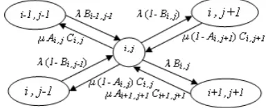
In this section, we develop the required Markovian balance equations for a specific values of thresholds. In order to clarify the balance equation, all possible transitions for (i,j) are shown in Figure 1.

The general detailed balance equation can be written as follows:

(1)



























 































B





F



i j

B F G E C A µ D E C A µ F C A µ F G C A µ E B D E B j i j j i j i j i j i j i j j i j i j i i j j i j i ij j ij ij j i ij ij j ij i j ij , 1 1 1 1 1 1 1 1 1 1 1 1 1 1 1 1 1 1 1 1 1 1 1 1 1 1 1 1 1 1 1                                                

This equation holds for any

w

w

w

i



c

,

c



1

,



,

and

j



0

,

1

,



,

k

. where

(2)













otherwise

L

i

j

if

A

ij

0

1

Figure 1. All possible transitions for (i,j) where wc< i < w

(3)













otherwise

U

i

j

if

B

_ij

0

1

(4)

) , ( min i j Cij 

(5)











otherwise

w

i

if

D

_i

0

1

(6)











otherwise

j

if

F

_j

0

0

1

(7)











otherwise

k

j

if

E

_j

0

1

(8)











otherwise

w

i

if

G

_i c

0

1

The left hand side of equation (1) represents the average transitions from state (i, j). The first two terms in the bracket specify the transitions due to receiving demand, Specifically with switching worker from NC to CCR and not respectively. The last two terms in the bracket specify the transitions due to satisfying demand, Specifically with switching worker from CCR to NC and not respectively. Also the right hand side of equation (1) represents the average transitions into state (i, j). The first two terms denote the transitions due to satisfying demand. Specifically, with switching worker from CCR to NC and not respectively. The last two terms indicate the transitions due to receiving demand. Specifically, with switching worker from NC to CCR and not respectively.

A

ij and

B

ij state whether the ratio of j (number of demands at CCR) to i (number of workers at CCR) is less than or equal to U and the ratio of j to i is greater than or equal to U , respectively.

C

ij is minimum of i and j.

D

_i and

G

_i state whether the number of workers at CCR is equal to w and

w

_c,

respectively. Besides,

F

_j and

E

_j state whether the number of demands at CCR is equal to zero and k, respectively. To find the steady-state probabilities for a specific value of thresholds, we can solve the corresponding system of linear equations, which contain the balance equations given in equation (1), and the normalizing constraint:

(9)

1

0





  w

w i

k

j ij

c



3.3 NC constraint

For the NC, we must have sufficiently many workers there (on average) so that the NC due to switching workers stays non-constraint and switching worker can’t make this NC into a bottleneck resource. Therefore, we require that the time-average worker complement in the NC to be equal or exceeds some minimum specified threshold.

(10)

0

w

w

nc



The time-average number of workers at NC is (11)

c

nc

w

w

w





(12)



 



w

w i

i c

c

i

w



(13)



 





w

w i

i nc

c

i

w

w



where the “dot” (•) notation signifies summation over all values of the missing index.

3.4 Objective function and optimization

problem

Every system has at least one bottleneck which limits the system's ability to improve its goal.

(14)



 



w

w i

k

j

ij ij

c

C

output

0





s.t. (1) - (10)

3.5 Model with no cooperation

If there is no switching of workers (CCR and NC are separate non-interacting stations), then CCR can be regarded as the

M

/

M

/

w

_c

/

k

queueing system, which has a finite capacity of size k and

c

w

servers. Demands arrive to the CCR in a Poisson manner with rate



demands/hour. Operations at CCR are done independently with exponential operation times in which mean operation time equal to



1. steady-state probability of the system being in state j (number of demands at CCR) is denoted herein by



j and written as follows [17]:

(15)

1 1

1 0

1 ! 1 !

1 1



 



 

   

  

      

      







k

w n

n

w n c c n

w

n c

c c

w w

n 

 

 

(16)

      

  

    

   

    



 ifw j k

w w

w j if j

c w

j c c j

c j

j

c 0 0

1 ! 1

1 0

! 1

 

   



In addition, CCR output is written as follows: (17)



 k

j

j j w_c C 0





4. HEURISTIC ALGORITHM

The following three conjectures are used in our heuristic to limit two thresholds that will be considered:

Conjecture 1. Increasing upper threshold decreases CCR output but also increases time-average NC manpower.

Conjecture 2. Increasing lower threshold decreases CCR output but also increases time-average NC manpower.

Conjecture 3. If for LL₁ and U U₁, the time-average worker is less than

w

0 , then there exists

no feasible solution for LL1 and U U2 or 2

L

L and U U₁ where L₂L₁ and U₂ U₁. Conjecture 1 states that, a policy that pulls workers from the NC at a large threshold will result in decreased CCR output but also better time-averaged manpower in the NC. Conjecture 2 states that, allowing workers to stay shorter in the CCR before switching to the NC provides less output CCR and thus the NC will “get better” in terms of time-average NC manpower. Conjecture 3 state that, decreasing lower or upper threshold decreases time-average NC manpower.

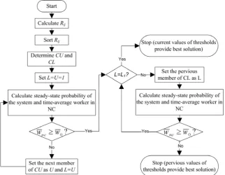
Our proposed algorithm solves the problem as follows:

Step 1: Calculate the

R

_ij ratio as follows:

i

j

R

_ij



where

i



w

_c

,

w

_c



1

,



,

w

and

j



0

,

1

,

2

,



,

k

.

Step 2: Sort values in ascending order of

R

_ij

with no repetitions and call them

R

1

,

R

2

,



,

R

m.

Step 3: Determine

CU





U

₁

,

U

₂

,



,

U

_n







Rt t 1,2,...,m



,

n



m

where CU is the set of

candidate values for the upper threshold with

1



t

R

.

Step 4: Determine

CL





L

₁

,

L

₂

,



,

L

_m







R_t t 1,2,...,m



, where CL is the set of candidate values for the lower threshold.

Step 5: Set

L



1

andU U1 1.

Step 6: Calculate steady-state probability of the system and time-average worker in NC. If the time-average worker is greater than or equal to

w

₀

go to step 7 (current solution is a feasible solution) else set the next member of CU as U and L=U, repeat step 6.

Step 7: If L is equal to L₁ stop and the current values of thresholds provide best solution else set the pervious member of CL as L; calculate steady-state probability of the system and time-average worker in NC.

If the time-average worker is greater than or equal to

w

0 repeat step 7 else stop and the pervious

values of thresholds provide best solution.

A flow chart of the heuristic method is included in Figure 2.

5. EXAMPLE

To illustrate the steps described in the previous section, consider the following example:



12,

4





,

w

₀



0

.

6

, k 5, w3 and with two dedicated workers in the CCR. The algorithm solves the problem as follows:

Step 1:

R

_ijratio is shown in Table 1.

Step 2: Sort values in ascending order of

ij

R

and call them

R

₁

,

R

₂

,



,

R

_m.

0

1

3

1

2

2

3

1

4

3

3

2

5

3

2

5

2

1

R R2

R

3 R4

R

5

R

6

R

7

R

8

R

9

R

10

Step 3: Determine the set of candidate values Table 1.

R

_ijratio

5 4 3 2 1 0 j i

2

5

2

2

3

1

2

1

0 2

3

5

3

4

1

3

2

3

1

0 3

for the upper threshold.







,

2

,

5

2



3

5

,

2

3

,

3

4

,

1

,

,

,

,

,

2 3 4 5 6

1





CU

U

U

U

U

U

U

CU

Step 4: Determine the set of candidate values

for the lower threshold.







,

2

,

5

2



3

5

,

2

3

,

3

4

,

1

3

2

,

2

1

,

3

1

,

0

,

,

,

,

,

,

,

,

,

2 3 4 5 6 7 8 9 10

1





CL

L

L

L

L

L

L

L

L

L

L

CL

Step 5: Set

L



1

andU U₁ 1.

Step 6: Calculate steady-state probability of the

system and time-average worker in NC.

According to the section 3.2, we write balance equations for current values of thresholds as follows:

12



₂₀



4



₂₁

16



₂₁



12



₂₀



8



₂₂

20



₂₂



12



₂₁



12



₃₃

24



₃₃



12



₂₂



12



₃₄

24



₃₄



12



₃₃



12



₃₅

12



₃₅



12



₃₄

To find the steady-state probabilities for current values of thresholds, we solve the corresponding system of linear equations, which contain above equations and the normalizing constraint:



₂₀





₂₁





₂₂





₃₃





₃₄





₃₅



1

Steady-state probabilities for current values of thresholds are:

0.0455

20





,



₂₁0.1364,



₂₂0.2045,

0.2045

33





,



₃₄



0.2045

and



₃₅



0.2045

.

Thus, the time-average worker complement in NC is calculated as follows:



 





w

w i

i nc

c

i

w

w



3

0.3864

3

2









  i

i

nc

i

w



The time-average worker less than

w

₀



0

.

6

, therefore set the next member of CU as U (U U₂ 4/3) and

L



L

₆



4

/

3

; repeat step 6. Summary of step 6 is shown in Table 2.

When LU 5/3, the time-average worker is greater than

w

₀. Therefore, we go to step 7. Step 7: Set

L



L

₇



3

/

2

; calculate steady-state probability of the system and time-average worker in NC. The time-average worker is greater than

w

₀, therefore repeat step 7. Summary of step 7 is shown in Table 3.

When

L



1

and U 5/3 , the time-average is less than

w

₀. Therefore, The algorithm stops and the pervious values of thresholds (L4/3 and

3 / 5 

U ) provide best solution. It means whenever

R

ij ratio is greater than or equal to5/3, the number of active CCR workers are increased from i to i+1 (for i2;

j



0

,

1

,

2

,

3

,

4

,

5

) and whenever

R

_ij ratio is less than or equal to 4/3, the number of active CCR workers are decreased from i to i1 (for i3;

j



0

,

1

,

2

,

3

,

4

,

5

).

The optimum output is calculated as follows:



 



w

w i

k

j

ij ij

c

C

output

0







20 21 22 23 24 34 35



3

2 5

0

3

3

2

2

2

1

0

)

4

(

)

4

(



































 

i j

ij ij

C

output

8.9094



output

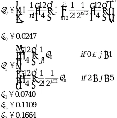
1 5 2 2 0 4 12 2 1 ! 2 1 4 12 ! 1 1                        



n n n n n





0 0.0247



















































2

5

2

1

!

2

1

4

12

1

0

!

1

4

12

0 2 0

j

if

j

if

j

j j j j









10.0740



₂ 0.1109



3



0.1664



₄ 0.2496



5



0.3744

CCR output is calculated as follows:



  5 0 ) 4 )( , 2 min( j j j output





 

 





 

 







































3744

.

0

2

2496

.

0

2

1664

.

0

2

1109

.

0

2

0740

.

0

1

0247

.

0

0

)

4

(

output

output



7.5069

Our heuristic method identifies an output of 8.9094. The total output for this problem assuming no cooperation (

M

/

M

/

w

_c

/

k

queueing system) Table 2. Summary of step 6

L steady-state U probabilities nc

w

1 1



20



0.0455

,



21 0.1364,



22 0.2045,



33



0.2045

,

0.2045

34





,



₃₅



0.2045

0.3864 (infeasible)

3

4

3

4



20



0.0348

,



21 0.1043,



22 0.1565,



23



0.2348

,

0.2348

34





,



₃₅



0.2348

0.5304 (infeasible)

2

3

2

3



20



0.0348

,



21 0.1043,



22 0.1565,



23



0.2348

,

0.2348

34





,



35



0.2348

0.5304 (infeasible)

3

5

3

5



20



0.0282

,



21 0.0845,



22 0.1268,



23



0.1901

,

0.2852

24 



,



35



0.2852

0.7148 (feasible)

Table 3. Summary of step 7

L steady-state U probabilities

w

e

2

3

3

5



20



0.0318

,



210.0954,



22 0.1431,



23



0.2146

,

0.1288

24 



,



₃₄



0.1288

,



₃₅



0.2576

0.6137 (feasible)

3

4

3

5



20



0.0318

,



210.0954,



22 0.1431,



23



0.2146

,

0.1288

24 



,



₃₄



0.1288

,



₃₅



0.2576

0.6137 (best solution) 1

5

3



20



0.0371

,



21 0.1112,



22 0.1668,



23



0.1317

,

0.0790

24 



,



33



0.0790

,



34



0.1580

,



35



0.2371

is 7.5069.

The above example shows that the heuristic method solution exceeds

M

/

M

/

w

_c

/

k

queueing system output by an additional 1.4025, which is a 19% increase over

M

/

M

/

w

_c

/

k

queueing system output.

6. COMPUTATIONAL RESULTS

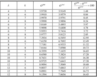
For the example discussed in the previous section, consider the following sets of parameter values:

8

7

,

6

,

5

;

12

10

,

8

,

6

,

4

and

k



and





. Table 4

contains the results of all combinations of



and k values. The third column of the table contains the output obtained from heuristic method (

O

HM ). The fourth column contains

O

NoC, total output

assuming no cooperation (

M

/

M

/

w

_c

/

k

queueing system). The fifth column provides the percentage that output of heuristic method over the no-cooperation solution.

Several conclusions can be drawn from Table 4:

 Our heuristic method clearly performs better than

M

/

M

/

w

_c

/

k

queueing system.

 By increasing of



and keeping other characteristics as constant, the output obtained from our heuristic method and

M

/

M

/

w

_c

/

k

queueing system will be increased.

 By increasing of k and keeping other characteristics as constant, the output obtained from our heuristic method and

M

/

M

/

w

_c

/

k

queueing system will be increased.

Table 4. Results of the example for variety of



and k values



k HM

O

O

NoC



_NoC



100

NoC HM

O

O

O

4 5 3.9730 3.9149 1.48

4 6 3.9910 3.9579 0.84

4 7 3.9970 3.9791 0.45

4 8 3.9990 3.9896 0.24

6 5 5.8169 5.4893 5.97

6 6 5.9098 5.6400 4.78

6 7 5.9553 5.7416 3.72

6 8 5.9777 5.8123 2.85

8 5 7.3934 6.5455 12.95

8 6 7.6150 6.7692 12.49

8 7 7.7181 6.9333 11.32

8 8 7.8164 7.0588 10.73

10 5 8.3559 7.1635 16.65

10 6 8.6580 7.3824 17.28

10 7 8.7631 7.5347 16.30

10 8 8.9725 7.6443 17.38

12 5 8.9094 7.5069 18.68

12 6 9.0037 7.6843 17.17

12 7 9.0991 7.7949 16.73

7. CONCLUSION

This paper proposed a policy for managing the system constraint. A model was developed based on that policy and heuristic algorithm was suggested to solve this model. The proposed heuristic algorithm compared with

M

/

M

/

w

_c

/

k

queueing system. The computational results indicate that the proposed algorithm clearly performs better than

M

/

M

/

w

_c

/

k

queueing system.

8. REFERENCES

1. Goldratt, E. M. and Cox, J., “The Race”, New York, North

River, (1986).

2. Goldratt, E. M., “The Haystack Syndrome: Sifting Information from the Data Ocean?”, New York, North River, (1990).

3. Goldratt, E. M., “Theory of Constraints: What Is This Thing Called the Theory of Constraints and How Should It Be Implemented?”, New York, North River, (1990). 4. Goldratt, E. M., Fox, R. E., “The Race”, New York,

North River, (1986).

5. Dettmer, H. W., “Breaking the constraints to world-class performance” Milwaukee, ASQ Quality, (1998).

6. Goldratt, E. M., “It’s Not Luck”, New York, North River, (1994).

7. Goldratt, E. M., “The goal”, New York, North River, (1984).

8. Buxey, G., “Production scheduling: Practice and theory”,

European Journal of Operational Research, Vol. 39,

(1989), 17–31.

9. Plenert, G., “Optimized theory of constraints when multiple constrained resources exist”, European Journal of Operational Research, Vol. 70, No. 1, (1993), 126– 133.

10. Luebbe, R. and Finch, B., “Theory of constraints and linear programming: a comparison”, International

Journal of Production Research, Voll. 30, No. 6,

(1992), 1471–1478.

11. Lee, T. N. and Plenert, G., “Optimizing theory of constraints when new product alternatives exist”,

Production and Inventory Management Journal, Vol.

34, No. 3, (1993), 51–57.

12. Fredenall, L. D. and Lea, B. R., “Improving the product mix heuristic in the theory of constraints”, International Journal of Production Research, Vol. 35, No. 6, (1997), 1535–1544.

13. Aryanezhad, M. B. and Komijan, A. R., “An improved algorithm for optimizing product mix under the theory of constraints”, International Journal of Production Research, Vol. 42, No. 20, (2004), 4221–4233.

14. Tsai, W. H., and Lai, C. W., and Chang, J. C., “An algorithm for optimizing joint products decision based on the Theory of Constraints”, International Journal of Production Research, Vol. 45, No. 15, (2007), 3421– 3437.

15. Bhattacharya, A., and Vasant, P., and Sarkar, B., and Mukherjee, S.K., “A fully fuzzified, intelligent theory-of-constraints product-mix decision”, International Journal of Production Research, Vol. 46, No. 3, (2008), 789-815.

16. Wang, J. Q., and Sun, S. D., and Si, S. B., and Yang, H. A., “Theory of Constraints product mix optimization based on immune algorithm”, International Journal of Production Research, Vol. 47 No. 16, (2009), 4521-4543 17. Askin, R. G. and Standridge, C. R., “Modeling and