Comparison of using Different Modeling Techniques on the Prediction of the Nonlinear Behavior of R/C Shear Walls

(1)

International Journal of Engineering

J o u r n a l H o m e p a g e : w w w . i j e . i r

Comparison of using Different Modeling Techniques on Prediction of the Nonlinear

Behavior of R/C Shear Walls

P A P E R I N F O

Paper history: Received 16 January 2013

Received in revised form 19 August 2013 Accepted 22 August 2013

Keywords:

Concrete Shear Walls RC Walls

Nonlinear Behavior Finite Element Model

A B S T R A C T

Reinforced concrete shear walls have been used throughout the world as known resisting elements for the lateral wind and earthquake loads. They are mostly designed and constructed based on elastic calculations and therefore resulting in un-economical sections. In order to overcome this weakness, scientists have proposed different methodologies to account for the non linear behavior of these walls. However, using these different models, different results are obtained causing doubts about the domain of their usage. In this paper, three known methods are used for the prediction of the non linear behavior of R/C shear walls and then they are compared to finite element one; investigating possibilities and weakness of each method. In doing so, first a nonlinear finite element model has been generated for a quarter-scale wall specimen and verified by an experimental model and then applied as a basis of the comparison to the used analytical models. Results are compared and relatively good agreements are obtained amongst three modeling methods with finite element one. Thereafter, methods used, procedure, modeling and the analytical results are presented in this paper.

doi:10.5829/idosi.ije.2014.27.02b.11

1. INTRODUCTION1

In order to design an economical R/C shear wall, it would be appropriate to utilize the non linear behavior of these walls. The accurate evaluation of this nonlinearity requires close attention to the important behavioral features such as tension-stiffening, non linearity and the axial force effect on the strength and stiffness [1].

In view of that, there are various models developed for the assessment of this nonlinear behavior. One method of nonlinear behavior estimation for R/C shear walls offered in 1988 by Ghobarah and Youssef [2] as illustrated in Figure1. In this model, the plastic zone of the wall is defined by the use of four steel and concrete springs. The boundary elements of the wall and its web element are also modeled with two outer and inner springs, respectively as shown.

Another practical approach on the inelastic behavior evaluation of the reinforced concrete shear walls, the equivalent reinforced concrete strategy, which has been

1_*_{Corresponding Author Email:}_{[email protected]}_{(F. Nateghi)}

depicted in Figure 2, suggested by Mazars et al. [3] in 2002. As the basis of framework method [4], this model utilized a lattice mesh to aid the evaluation of the nonlinear behavior of the shear walls. The fundamental idea of the framework method consisted in replacing the continuum material of the elastic body under investigation with a framework of bars was arranged according to a definite pattern, whose elements had appropriate elastic properties. 1-D constitutive law [5, 6] was handled for the concrete and steel materials.

Moreover, in 2006, Orakal and Wallace [7] postulated another beneficial strategy that revealed detailed information on the calibration of MVLEM by comparing the analytical results with the experimental results for the reinforced concrete walls with rectangular and T-shaped cross sections.

Figure 3 shows a structural wall which was modeled as a stack of m-elements, which were placed one upon the other. The flexural response is simulated by a series of n-uniaxial elements connected to infinitely rigid beams at the top and bottom levels.

Eventually, Belmouden and Lestuzzi [8] in 2006 advocated an inelastic one-dimensional finite element

O. Saghaeiana, F. Nateghi* b, O. Rezaifar

b International Institute of Earthquake Engineering and Seismology, Tehran, Iran a Department of Civil Engineering, Azad University South of Tehran Branch, Tehran, Iran

Faculty of Civil Engineering Department, Semnan University, Iran

c

c c

(2)

model for a seismic two dimensional frame analysis. As shown in Figure 4, it consisted of multi-layered Timoshenko beam-elements coupled with the fiber connection hinges, which were two multilayer finite interfaces with zero length and two degrees of freedom. Taking into consideration the deformations that occur in the beam-to-column, column-to-footing or wall-to-footing connections, the fiber connection hinges should be specified at the beam ends. To characterize the constitutive laws of the layers, uniaxial stress–strain relationships should be simultaneous with shear stress–

strain relationships for the beam elements.

It should be highlighted that there are widespread experimental evidences which indicate that diverse issues affect the nonlinear behavior of the shear walls. The monotonic loading tests on slender reinforced concrete shear walls validated that concentration and appropriate confinement of the longitudinal reinforcements in the boundary elements of the R/C walls extended their ductility [9]. Not only, this valuable insight provide in the monotonic loading tests, but also the aforesaid improvements have been confirmed in the cyclic ones as well [10, 11]. Another contributing factor that influences the nonlinear behavior of the shear walls is diagonal web reinforcement which was investigated by Sittipunt [12] in 2001.

Figure 1. A. Ghobarah and M. Youssef model [2]

Figure 2. Reinforced concrete equivalent model (ERC) [3]

Figure 3. Multiple-vertical-line-element model [7]]

Figure 4. Multilayer finite element model [8]

This paper motivates by establishing the validity of the analytical model which is implemented in the ABAQUS. In this way, the correlation between the analytical results in ABAQUS and the experimental results obtained by Thomsen and Wallace are studied [13]. Afterwards, the exactness of the column analogy, truss analogy and fiber element modeling approaches are compared with the finite element model. Comparisons are carried out not only to comprehend the nonlinear behavior of the R/C shear walls, but also to discern the capability of the models and the techniques to improve them.

2. EXPERIMENTAL AND ANALYTICAL RESULTS FOR A QUARTER-SCALE WALL SPECIMEN

(3)

by ACI318-19 code [16]. Reinforcement details for the wall specimen are shown in Figure 5.

An axial force was applied at the top of the wall by a hydraulic actuator and held constant during the test. Cyclic lateral displacements were applied to the wall by means of a hydraulic actuator mounted horizontally on the wall. To prevent twisting of the wall specimen for the duration of the test, out of plane support was provided. Given analytical wall specimen that was implemented in ABAQUS were subjected to horizontal displacement up to the target point; the monotonic enveloped curve of the experimental load-deformation should drawn special attention. Figure 6 depicts the load-displacement diagram from the experiment. The concrete and reinforcement properties are summarized in Table 1 and 2 [7, 13].

2. 2. Analytical Results As the finite element technique is a numerical progression to resolve the differential equations, it can provide engineers with valuable insight into the behavior of the structural elements. This section employs ABAQUS to reproduce the nonlinear behavior of a reinforced concrete wall specimen. ABAQUS is a robust analytical tool used for element and structural modeling and also has been widely applied in a variety of fields. Taking advantage of the ability of ABAQUS to represent the nonlinear behavior of materials, the concrete and steel relations will be characterized later.

This program has a broad range of elements and the key issue here would be the selection of an appropriate element type based on the problem. In this case, the four-node shell elements are preferred by virtue of the displacement and rotational degrees of freedom in order to model the reinforced concrete shear wall under the seismic loads [16]. These elements are utilized to represent structures in which one dimension, the thickness, is considerably smaller than the other dimensions. Actually, the shell elements discretize a body by defining the geometry at a reference surface, and the thickness is defined through the section property definition. Figure 7 exhibits the discretization of the wall cross section by means of shell elements. Precise recreation through a computational attempt necessitates the properties of the materials involved, to be modeled

as close to the physical specimen as plausible. In this regard, the stress-strain relations of the reinforcements were defined by means of kinematic hardening model [17] which was presented in the documentation of ABAQUS; in fact, it is a cyclic model which can take into account the Bauschinger effect and the buckling. As input data in ABAQUS, the stress and the strain at the yield point and at an arbitrary point were given. The parameters utilized for modeling of the steel stress-strain relations in ABAQUS are presented in Table 3 and 4. [7]

Figure 5. Wall cross section [7]

Figure 6. Comparison of analytical and experimental load-deformation responses [7]

TABLE 1. Concrete properties [7]

Concrete properties Elastic modulus of Concrete (GPa) Compressive strength (MPa)

Boundary (confined concrete) 31.03 47.60

Web (unconfined concrete) 31.03 42.80

TABLE 2. Steel properties [7]

Steel properties Elastic modulus of steel (GPa) Yield stress ( MPa)

#3 reinforcing bars (_d_b=_9.53_mm) ₂₀₀ ₃₉₅

(4)

TABLE 3. Modeling parameters for #3 bars [1]

Point of stress-strain curve Modulus of elasticity (GPa) Stress (MPa) Plastic strain

Start yielding point 200 395 0.00000

Arbitrary point beyond yielding 200 398.79 0.00097

TABLE 4. Modeling parameters for #2 bars[1]

Start yielding point 200 336 0.000000

Arbitrary point beyond yielding 200 345.24 0.001215

Figure 7. Modeling of the R/C wall using 4-node shell elements [1]

Figure 8. Hoshikuma concrete constitutive model [19]

Figure 9. Applied displacement history [29]

To characterize the concrete stress-strain relations, Concrete Damage Plasticity model [17, 18] which was implemented in ABAQUS documentation is utilized. One of the possible advantages of this strategy is the assessment of the wall behavior based on the progression of the damage in the concrete. This requires an estimate of the variation of the accumulated damage with respect to the strain in concrete. If a chosen material model is unable to map such feature, the structural response will be imprecise. Indeed, the Concrete Damage Plasticity model incorporates the behavior of concrete in both tension and compression and also the significant features of the behavior such as hardening, softening and stiffness degradation effects in the concrete. Furthermore, modeling the wall specimen ties in ABAQUS, Hushikuma unconfined concrete relations [19, 20] were applied to generate the values of stress and strain of this model. The required relation for the estimation of plastic strain besides the concrete stress-strain relations which was proposed by Hoshikuma will be then briefly addressed.

The applied displacement history on the top of the wall has been depicted in Figure 9. As well, from the comparison between the analytical and experimental load-deformation responses, reasonable agreement with the experimental results is obvious (Figure 10). It should be stated that larger analytical load-deformation values may be due to the fact that experimental results which were represented by Thomsen and Wallace [13] have been investigated under the cyclic loading, whereas the analytical diagram has been provided through monotonic loading in ABAQUS. This accommodates the test results of Portland cement in which fifty percent degradation of the flexural strength under the cyclic loading as well as the slow increase in the amplitude of the loading are observed as compared with monotonic load [10, 11].

2. 3. Hoshikuma Concrete Constitutive Model As previously mentioned, Hoshikuma [19] constitutive model has provided the plastic strain values for the concrete. In continuation, various parameters associated with this model in the compression and tensile region 0

1 2 3 4 5 6

0 5 10 15

Time(s)

T

op

L

at

er

al

D

is

pl

ac

em

en

t(

in

(5)

are shown in Figure 8. The parameters of the concrete compression region are the compressive stress_f_cc, the corresponding strain e_cc, the ultimate strain of confined concrete e_cu, the compressive stress in unconfined concrete f_co, and the corresponding straine_co. The

parameters of the concrete tensile region are the concrete tensile stress f_t¢ and the ultimate tensile strain

tu

e . Initial slope of the curve E_c postulated in both

tensile and compressive behaviors are identical. Moreover, the relationshipof Hoshikuma constitutive model is characterized as follows:

Concrete in compression: -Ascending branch:

1 1

n c

c c c

c c f E n e e e

é _æ _ö ù

ê ú

= - _ç _÷

ê è ø ú

ë û (1)

-Descending branch:

( )

c c c de s c c c

f = f -E e -e (2)

c cc c cc cc

E n E f e e = - (3) resid cc cc des cu cc

f

E

e

-= - (4) 1.4

0 .004 sh yh su h

cu

cc f f

r e

e = + (5)

3.8

cc co sh yh

f = f + a r f (6)

0.002 0.033 sh yh

cc

co f f

r

e = + b (7)

According to Mender constitutive model [21] r_sh,

suh

e , and f_yh are respectively the volumetric ratio, the ultimate strain and the yield strength of the transverse reinforcement. As well, a and b are the cross section coefficients. It should be noted that for the circular sections, a =b =1 and for square sections, a=0.2 and

0.4

b = . In this way, to avoid the numerical problems, 0.2fcc is considered as a residual value of the confined concrete strength. The plastic strain for ABAQUS calculations are given by [22]:

2

0.145( ) 0.13( )

p c c

cc cc cc

e e e

e = e + e (8)

The unconfined concrete constitutive model consists of a nonlinear ascending branch and a linear descending branch (Figure 8). The relationships for these branches in both unconfined concrete and confined concrete are similar except that f_cc and

e

_{c c} which are replaced with

co

f

and

e

_{c o}(Equations (1), (3) and (8)), respectively and E_des is given by E_des =f_co/ 2e_co. In this paper,

0.85

co c

f = f¢ and f_c¢is the compressive strength of concrete from the standard compressive test in terms of MPa.

e

_{c o}is taken as 0.002. The bilinear constitutive model which represents the confined and unconfined concrete in tension is shown in Figure 8.

Concrete in tension [17, 19]:

0 .1

t c

f ¢ = f (9)

t t

c

f E

e = ¢ (10)

Figure 10. Analytical and experimental load-deformation responses [29]

3. FINITE ELEMENT AND STRAIGHTFORWARD STRATEGIES RESULTS FOR A REALISTIC-WALL SPECIMEN

The comparison of the analytical and experimental results for the quarter-scale wall specimen substantiated the capability of employed analytical model in ABAQUS besides Hoshikuma [19, 20] relations to predict the accurate wall responses. Owing to this good agreement, those can be utilized as a basis for other analytical wall models with different compressive strengths and dimensional characteristics. In the following, another wall specimen will be considered. At first, aforesaid realistic wall specimen has been designed; after that, it has been analyzed by three

0 5 10 15 2 0 25 3 0 35 4 0

0 0.5 1 1.5 2 2 .5 3 3 .5 4

T op Lateral Displacement(inch)

L at er al L oa d( k ip

s) _{T est}

(6)

simplified analysis strategies and also compared with finite method.

3. 1. Desgin of the Realistic Wall Specimen The realistic wall specimen was 4 m tall and 0.3 m thick. Typical material properties were selected for design, i.e.

2

210 /

c

f¢ = kg cm and 2

4000 /

y

f = kg cm . The exhaustive material properties of the wall specimen are summarized in Table 5.

Initially, a prototype residential building in the high seismic risk area was employed to assess the wall geometry and the reinforcing details (Figure 11) [23]. The prototype building was a three story building with a total height of 9 m and incorporated rectangular walls, besides moment resisting frames to cope with the lateral and gravity loads. Then, to design the wall specimen, which is illustrated in Figure 11, the three-dimensional model of the building was built via ETABS 9.5.0.

It should be noted that gravity loads of the building were evaluated based on Iranian National Building Code [24] and also its seismic loads were estimated based on 2800 ,3nd _{, standard code. By the way, taking}

the advantage of the ultimate strength design methodology in ACI318-95 [16], the detailing requirements were determined for the wall specimen (Figure 12). The boundary vertical steels consist of

8-18

f (d_b =18mm) bars, while the web bars compose of 14

f (d_b =14mm) bars. Additional information are illustrated in Figure 12.

Figure 11. Building plans (based on meter) [1]

Figure 12. Reinforced concrete shear wall model [1]

TABLE 5. Concrete and steel properties Properties

2400 Density(kg/cm3₎

230017 Modules of elasticity for _0.5f_c¢stress (kg/cm2₎

0.2 Poison coefficient

210 Compressive strength of concrete (kg/cm2₎

4000 Yield stress of longitudinal steel (flexural) (kg/cm2₎

4000 Yield stress of transverse steel (kg/cm2₎

3. 2. Analysis Method The realistic wall specimen is analyzed by the nonlinear static analysis approach, also named pushover analysis, which is a simplified analytical strategy for the performance evaluation of buildings under seismic loads. In this approach, a monotonically increasing lateral load is statically applied to the structure until the target displacement at the certain point (control point), is exceeded or the structure is collapsed. At the outset, given the Seismic Rehabilitation of Building Code [25] requirements, one of the three following lateral load patterns should be underlined:

1. A vertical distribution which is proportional to vertical distribution of linear static method. Use of this distribution shall be permitted only when more than 75% of the total mass participates in the fundamental mode in the direction under consideration, and the uniform

distribution is also used.

2. A vertical distribution which is proportional to the shape of the fundamental mode in the direction under consideration. Use of this distribution shall be permitted only when more than 75% of the total mass participates in this mode.

(7)

of the shear wall is also regarded at the Life Safety Performance Level.

Finally, the effects of the upper and lower limits of the gravity loads in the combinations of the gravity and lateral loads are assessed from the following relations using seismic rehabilitation of building code:

1 1.1( ), 2 0.9

G D L G D

Q = Q +Q Q = Q

QD = Dead-load QL = Effective live load

SPUY= The upper limit of gravity load combination + the vertical distribution proportional to the story shear distribution calculated from a response spectrum analysis

SPLY= The lower limit of gravity load combination + the vertical distribution proportional to the story shear distribution calculated from a response spectrum analysis

It should be stated that in present paper, the upper limit of gravity load combination has been studied.

3. 3. Finite Element Model The realistic wall specimen was implemented in ABAQUS to draw a direct comparison between the results of the finite element method and three simplified modeling approaches. Again, the numerical analysis for the above wall specimen are performed via four-node shell elements in ABAQUS as those accomplished for the

quarter scale wall specimen (Figure 13). Concerning the material behaviors, the stress-strain relations of the concrete and reinforcement bars were performed using concrete damage plasticity [26, 27] and kinematic hardening model respectively in ABAQUS. In this regard, the required stress-strain values for the concrete damage plasticity model have been assessed based on the Hoshikuma unconfined concrete relations [19] same as the earlier sections. Before analysis, the analytical models were subjected to the dead and live loads which were the concentrated loads applied at the nodes of the floor level. Simultaneously, the weight of each element are estimated and imposed on the central point of the wall elements with regard to the material density in ABAQUS. Afterwards, the lateral load distribution, based on Table 7, is applied on the floor levels and also gradually increases until target displacement at the mass center of third floor is exceeded.

TABLE 7. Story force due to response spectrum analysis

Story Height (mm) Force (N)

STORY3 9000 165683.30

STORY2 6000 125286.00

STORY1 3000 72502.02

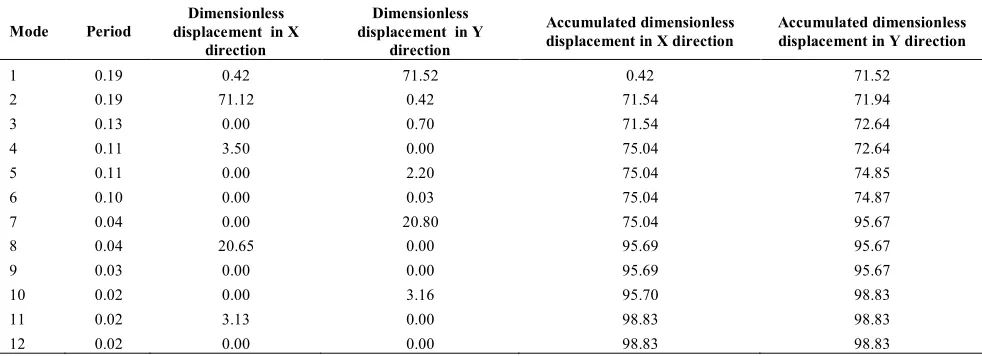
TABLE 6. The building modal information via ETABS

Mode Period displacement in X Dimensionless

direction

Dimensionless displacement in Y

direction

Accumulated dimensionless displacement in X direction

Accumulated dimensionless displacement in Y direction

1 0.19 0.42 71.52 0.42 71.52

2 0.19 71.12 0.42 71.54 71.94

3 0.13 0.00 0.70 71.54 72.64

4 0.11 3.50 0.00 75.04 72.64

5 0.11 0.00 2.20 75.04 74.85

6 0.10 0.00 0.03 75.04 74.87

7 0.04 0.00 20.80 75.04 95.67

8 0.04 20.65 0.00 95.69 95.67

9 0.03 0.00 0.00 95.69 95.67

10 0.02 0.00 3.16 95.70 98.83

11 0.02 3.13 0.00 98.83 98.83

12 0.02 0.00 0.00 98.83 98.83

TABLE 8. Target displacement [1]

Target displacement (mm) C0 C1 C2 C3 SA TE

14.10 1.20 1.39 1.25 1.00 0.75 0.19

TABLE 9. Modeling parameters for steel

Start yielding point 200 392.30 0.00000

(8)

Figure 13. Modeling via four-node shell elements

Figure 14. Unconfined concrete Hushikuma model

Figure 15. Column analogy method and assigned hinges

3. 4. Column Analogy Method The column analogy methodology is a frame based model which incorporates a set of frame elements. Based on the previous studies, a thin symmetrical wall with a height-to-length ratio greater than 2 can be assumed as a vertical cantilever on account of the fact that it is governed by the bending moment. The moment of inertia and the shear surface of the column in each zone is the same as the primary wall. Since the height-to-length ratio of the wall specimen is about 2.25, the column analogy method seems appropriate [28, 29].

It is essential to know that the nonlinearity of material in any frame element can be disclosed by either lumped [30] or the distributed plasticity model [31]. In the lumped plasticity model, a frame element is composed of two zero-length nonlinear rotational spring elements and an elastic element which connects them. The nonlinear behavior of structures is evaluated by nonlinear moment–rotation relationships of these spring elements. More specially, the lumped plasticity model is widely used in the high-volume analysis calculations such as nonlinear time-history analysis of a large structure due to effortlessness of this model [19].

The column analogy strategy is implemented the lumped [31] plasticity model at the critical sections (location where the yielding is expected like the critical flexural sections at the top and the bottom of story height and also the critical shear section at the middle of story height ), it also assumes that the rest of element remains perfectly elastic. Figure 15 details the two non-linear rotational springs (PMM) at the two ends of element together with the shear hinges (VHING) at the middle height of each story in SAP.

TABLE 10. Nonlinear flexural-axial hinges properties

Tw= 300 P/(TwLwfc)= 0.1 0.25

Lw= 4000 P= 2473200000 6183000

fc= 20.61 a= 0.0150 0.0090

b= 0.0200 0.0120

c= 0.7500 0.6000

TABLE 11. Nonlinear shear hinges properties VHING

Tw= 300 VC= 653734.63

Lw= 4000 VS= 1640624.40

fc= 20.61 V= 2294359.03

vc= 0.54 a= 0.75

A= 1200000 b= 2.00

FY= 392.50 c= 0.40

-5 -2.5 0 2.5 5 7.5 10 12.5 15 17.5 20

-0.002 -0.001 0 0.001 0.002 0.003 0.004 0.005 0.006 0.007

str

es

s(

mp

a)

(9)

In continuation, the properties of the flexural hinges in conjunction with the shear hinges have been defined by seismic rehabilitation of building code (Table 10 and 11). It should be mentioned that combination of the gravity loads, the lateral loads, and their distribution in the analysis of all later simplified schemes are the same as those in the analysis of the finite element method.

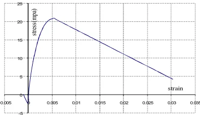
3. 5. Truss Analogy Method The truss analogy strategy is also a frame based model which incorporates a set of braced frame elements. Correspondingly, the cross section of the column is postulated as 25% wall’s cross section, yet the cross section of the brace elements has been estimated so that elastic lateral stiffness of the trusses and the shear walls are the same. The plastic moment arm of wall’s cross section is equivalent to the distance between two centers of the boundary elements in the horizontal plane (3200 mm). This value is adopted by ACI318-95 code regulations 11-10-4 [16] where the effective depth of shear is taken 0.8L, here L stands for the length of the wall.

In order to achieve a good compromise between the simplicity and the accuracy, a bilinear description is used in the axial hinges (Figure18). Relevant parameters to define this model such as the yield axial force, the plastic axial force and plastic deformation of the cross sections have been calculated through use of the moment and rotation values.

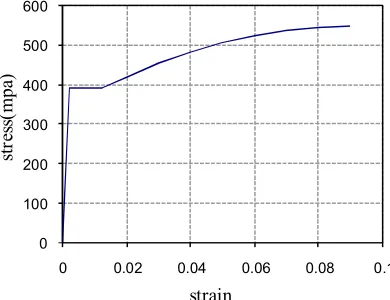
To evaluate the plastic moment of the wall, the moment-curvature curves obtained from the SAP software have been employed [32]. In this regard, the nonlinear behavior of the concrete materials in the boundary regions is assessed using confined concrete Hoshikama relations and at the web of the wall using unconfined ones (Figure 10), and the nonlinear behavior of the reinforcement bars has been estimated by the Equation (11)(Figure17):

2

( )( cu s ) ,

s u u y sh s su

su sh

f f f f e e e e e

e e

-= - - < <

- (11)

where,

f

_s,

e

_s,

f

_u,

e

_sh and

e

_su are respectively the steel stress, the steel strain, the ultimate stress, ultimate strain, the strain at the beginning of hardening, and ultimate strain. Regarding the dependence of the moment-curvature diagrams on the gravity load values, those should be computed in each floor level. It is to be noted that plastic moment of the cross-section occurs when the moment reaches its maximum point in Figure 20.

Nevertheless the plastic rotations,

q

_p , is evaluated based on the seismic rehabilitation of building code

provisions in case that [ s s ] y _0.1 w w c

A A f P

t l f

¢

- +

£

¢ , the slope

of the bilinear curve is equal to slope from point B to C

which is taken between zero to 10 percent of elastic slope (slope from point A to B) (Figure 21) [25].

Figure 16. Houshikuma confined concrete model

Figure 17. Steel constitutive model

Figure 18. Truss analogy method and assigned hinges

-5 0 5 10 15 20 25

-0.005 0 0.005 0.01 0.015 0.02 0.025 0.03 0.035

str

es

s(

m

pa)

(10)

Figure 19. Bilinear moment-rotation curve

Figure 20. Moment-curvature curve SPUY

Figure 21. Load-deformation relationship for the concrete element [25]

Figure 22. Subdivision of the cross-section of the wall to fiber elements [1]

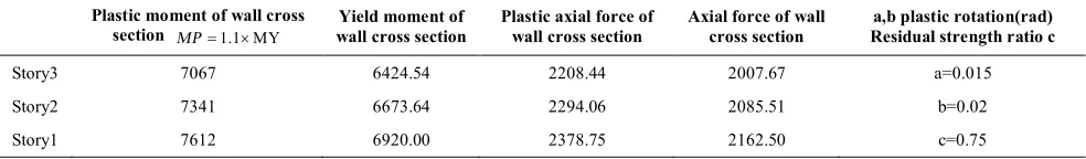
TABLE 12. Nonlinear axial hinges properties (N-mm) Plastic moment of wall cross

section MP=1.1 MY´

Yield moment of wall cross section

Plastic axial forceof

wall cross section

Axial force of wall cross section

a,b plastic rotation(rad) Residual strength ratio c

Story3 7067 6424.54 2208.44 2007.67 a=0.015

Story2 7341 6673.64 2294.06 2085.51 b=0.02

Story1 7612 6920.00 2378.75 2162.50 c=0.75

The shear behavior of the wall have been assumed in the elastic domain before the analysis, and afterwards the validity of the first postulation has been investigated through the estimation of the ratio of the existing shear force to the yield strength in each floor. In this way, as this ratio was less than one, the first assumption could be correct.

3. 6. Simulation with Fiber Element Simulation with the fiber element as the third method of the modeling shear walls in this part of the article will be considered. In this section, the perform-3D model will employ fiber cross-sections or what perform-3D labels as “shear wall elements” consisting of the steel and concrete fibers. The shear wall element not only is a macro-element with 4-nodes and 24 degrees of freedom, [33] but also defines the nonlinearity of the material by the distributed plasticity model [19]. See Figure 22 for a graphical representation of the steel and concrete fibers. However, the shear wall elements in PERFORM have the identical behavior with the deep beams and their out-of-plane bending is assumed to be elastic [20].

To begin, the wall specimen is divided by 50 × 50 cm shear wall elements (Figure 23) and also each shear wall element is subdivided into two concrete and steel fibers (Figure 22). Then the nonlinear behavior of the concrete and steel are assigned to the fibers. Since the transverse bars cannot be modeled in perform-3D, the confined concrete Hoshikuma model is implemented in the boundary elements of the wall, while the unconfined model is utilized in the web element (Figures 14 and 16). The nonlinear behavior of the steel is defined by the steel constitutive model which is depicted in Figure 24.

4. COMPARISON OF ANALYTICAL STATEGIES AND FINITE ELEMENT RESULTS

Figures 25-29 compare the ABAQUS results and three equivalent modeling approaches corresponding to the SPUY level of loading. Figure 25 compares the base shear profiles of various approaches, the following results have been achieved:

0 1000 2000 3000 4000 5000 6000 7000 8000 9000

0 5 10 15 20 25 30 35 40 45 50

m

om

en

t(

k

N

m)

curvature(rad/km)

(11)

1. It has been observed that simulation with fiber element method in comparison with the other ones is in good agreement with the finite element strategy. The pragmatic differences in the nonlinear region can be attributed to the uncertainty in the parameters associated with modeling the confined concrete relations. 2. Truss analogy method is more accurate by

virtue of the brace element which simulates the wall’s shear behavior in comparison with the column analogy strategy which cannot reproduce this behavior.

Figure 23. Modeling by four shear wall elements

Figure 24. Reinforcement constitutive model

Figure 25. Base shear profiles in SPUY combination

Figure 26. Load-deformation results in SPUY combination

3. Given the bilinear behavior which employed for the concrete material in the nonlinear hinges, the bilinear trend in the base shear- deformation diagram in the truss analogy and column strategies can be reasonable.

4. Results presented in Figure 25 also reveals that simulation with fiber element has the most precision among all strategies followed by truss analogy and column analogy, respectively.

As well, the following results are obtained by the comparison of the base shear stories graphs:

1. In simulation with fiber element at the second and third-story levels, which the base shear values cannot be captured with the finite element model, little discrepancies are beholden. Nevertheless, these values have 0

100 200 300 400 500 600

0 0.02 0.04 0.06 0.08 0.1

st

re

ss

(m

pa)

strain

0 3000 6000 9000 12000

0 200 400 600 800 1000 1200 1400

he

ig

ht

(mm)

shear(kN)

simulation with fiber element finite element

column analogy

truss analogy

0 200 400 600 800 1000 1200

0 2 4 6 8 10 12 14 16

sh

ea

r(k

N)

disp.(mm)

(12)

predicted almost similarly with finite element method in the first-story levels.

2. The exactness of predicted results resemble those discussed for above strategy.

In continuation, the predicted lateral deformations values of three approaches are in close agreement with the finite element one (Figure 27). In the long run, Figure 28 illustrates that the column analogy strategy has a good potential to provide precise prediction of the story drift values.

5. SUMMARY AND CONCLUSION

In this work, three simplified modeling approaches, which compared with finite element method, are characterized to simulate the nonlinear seismic response of R/C walls: column analogy, truss analogy, and simulation with fiber elements. The paramount virtue of them lies in their straightforwardness and the fast calculations for the official and commercial objectives, notwithstanding above approaches the finite element one is computationally more involved but it provides more precise values.

At the beginning, this article drew a comparison between the finite element model and the test results for a quarter-scale wall specimen. Given the exactitude of achieved results, this model was capable to predict the inelastic response of the R/C walls. Eventually, the results of three aforementioned models were compared with the finite element one for a realistic wall specimen. From the comparison, excellent agreement with the finite element was observable. As well, three important conclusions of general view could be drawn as follows:

Figure 27. Drift profiles in SPUY combination

Figure 28. Lateral displacement profiles in SPUY combination

Firstly, the estimated lateral deformations and the base shear values disclose that simulation with fiber element approach in comparison with other ones is the most precise and the column analogy strategy is the least one. The simulation with fiber element approach underestimates the finite element top displacements by up to approximately 9% in the regions where inelastic deformations are expected. However, the truss analogy method overestimates the finite element top displacements (by up to 18%), as well as those in column analogy technique (by up to 20 %.).

Secondly, the lateral deformations predicted by all above approaches are in good agreement with finite element one.

Thirdly, the column analogy strategy captures the finite element story drifts reasonably well. Nevertheless, the fiber element approach overestimates the story drifts at the second besides third floor, and underestimates them at the first floor. Likewise, the truss analogy approach overestimates the story drifts at the first floor level.

[1-32]

8. REFERENCES

1. A., S., Predicting nonlinear behavior of rc shear walls, in Civil Engineering Department., Azad University South of Tehran Branch (2010 ).

2. Ghobarah, A. and Youssef, M., "Modelling of reinforced concrete structural walls", Engineering Structures, Vol .21 , No. 10, (1999), 912-923.

3. Mazars, J., Kotronis, P. and Davenne, L., "A new modelling strategy for the behaviour of shear walls under dynamic loading", Earthquake Engineering & Structural Dynamics, Vol. 31, No. 4, (2002), 937-954.

0 3000 6000 9000 12000

0.04 0.06 0.08 0.1 0.12 0.14 0.16 0.18 0.2

he

igh

t (

mm)

drift(%)

simulation with fiber element finite element

column analogy

truss analogy

0 3000 6000 9000 12000

0 2 4 6 8 10 12 14 16

hei

gh

t(

mm)

displace ment(mm)

(13)

4. Hrennikoff, A" ,.Solution of problems of elasticity by the framework method", Journal of Applied Mechanics, Vol. 8, No. 4, (1941), 169-175.

5. Mazars, J., "A description of micro-and macroscale damage of concrete structures", Engineering Fracture Mechanics, Vol. 25 ,No. 5, (1986), 729-737.

6. La Borderie, C., " phenomenes unilateraux dans un materiau endommageable: Modelisation et application a l'analyse des structures en beton. Ph. D, universite paris 6",. (1991)

7. Orakcal, K. and Wallace, J. W., "Flexural modeling of reinforced concrete walls-experimental verification", ACI

Structural Journal, Vol. 103, No. 2, (2006).

8. Belmouden, Y. and Lestuzzi, P., "Analytical model for predicting nonlinear reversed cyclic behaviour of reinforced concrete structural walls", Engineering Structures, Vol. 29, No. 7, (2007), 1263-1276.

9. Cardenas, A. and Magura, D. D., "Strength of high rise shear walls rectangular cross section. Response of multi story concrete structures to lateral forces", ACI Publication SP-36, AmericanConcrete Inistitue, (1973)

10. Oesterle, R., "Earthquake resistant structural walls: Tests of isolated walls: Phase ii", Construction Technology Laboratories, Portland Cement Association, (1979)

11. Oesterle, R., "Earthquake resistant structural walls: Tests of isolated walls", Research and Development Construction Technology Laboratories, Portland Cement Association, (1976). 12. Sittipunt, C., Wood, S. L., Lukkunaprasit, P. and Pattararattanakul, P., "Cyclic behavior of reinforced concrete structural walls with diagonal web reinforcement", ACI

Structural Journal, Vol. 98, No. 4, (2001).

13. Thomsen IV, J. H. and Wallace, J. W., "Displacement-based design of slender reinforced concrete structural walls-experimental verification", Journal of Structural Engineering, Vol. 130, No. 4, (2004), 618-630.

14. Wallace, J. W., "New methodology for seismic design of rc shear walls", Journal of Structural Engineering, Vol. 120, No. 3, (1994), 863-884.

15. Wallace, J. W., "Seismic design of rc structural walls. Part i: New code format", Journal of Structural Engineering, Vol. 121, No. 1, (1995), 75-87.

16. ,٣١٨A. C. I. C., "Building code requirements for structural concrete (ACI 318-95) and commentary (ACI 318r-95)", American concrete institute. (1995 ).

17. Pawtucket, R., "Abaqus/analysis user’s manual—version 6.8",

ABAQUS, USA, (2008)

18. Hillerborg, A., Modéer, M. and Petersson, P.-E., "Analysis of crack formation and crack growth in concrete by means of fracture mechanics and finite elements", Cement and Concrete

Research, Vol. 6, No. 6, (1976), 773-781.

19. Lee, T.-H. and Mosalam, K. M., "Probabilistic fiber element modeling of reinforced concrete structures", Computers &

Structures, Vol. 82, No. 27, (2004), 2285-2299.

20. Hoshikuma, J., Kawashima, K., Nagaya, K. and Taylor, A., "Stress-strain model for confined reinforced concrete in bridge piers", Journal of Structural Engineering, Vol. 123, No. 5, (1997), 624-633.

21. Mander, J. B., Priestley, M. J. and Park, R., "Theoretical stress-strain model for confined concrete", Journal of Structural

Engineering, Vol. 114, No. 8, (1988), 1804-1826.

22. Noh, S.-Y., Krätzig, W. B. and Meskouris, K., "Numerical simulation of serviceability, damage evolution and failure of reinforced concrete shells", Computers & Structures, Vol. 81, No. 8, (2003), 843-857.

23. "Building and housing research center (BHRC), iranian code of practice for seismic resistant design of buildings, standard no. 2800-94, 3st edition, building and housing research center, (1994)

24. "Ministry of housing and urban development, iranian national building code-part 6", (2006)

25. "Instruction for seismic rehabilitation of existing buildings , no. 360 , management and planning organization , I.R.Iran", , (2007).

26. Lee, J. and Fenves, G. L., "Plastic-damage model for cyclic loading of concrete structures", Journal of Engineering

Mechanics, Vol. 124, No. 8, (1998), 892-900.

27. Lubliner, J., Oliver, J., Oller, S. and Oñate, E" A plastic- ,. damage model for concrete", International Journal of Solids

and Structures, Vol. 25, No. 3, (1989), 299-326.

28. Naeim, F., "The seismic design handbook", Springer, (1989) 29. Stafford Smith, B. and Coull, A., "Tall building structures:

Analysis and design", John Willey, New York, (1991). 30. D'Ambrisi, A. and Filippou, F. C., "Modeling of cyclic shear

behavior in rc members", Journal of Structural Engineering, Vol. 125, No. 10, (1999), 1143-1150.

31. Spacone, E., Filippou, F .C. and Taucer, F. F., "Fibre beam-column model for non-linear analysis of R/C frames: Part ii. Applications", Earthquake Engineering and Structural

Dynamics, Vol. 25, No. 7, (1996), 727-742.

(14)