Stiffness Prediction of Beech Wood Flour Polypropylene Composite by using Proper Fiber Orientation Distribution Function

(1)

Please cite this article as: R. Khamedi, I. Ahmadi, M. Hashemi, K. Ahmaditabar, Stiffness Prediction of Beech Wood Flour Polypropylene Composite by using Proper Fiber Orientation Distribution Function, International Journal of Engineering (IJE), TRANSACTIONS A: Basics Vol. 30, No. 4, (April 2017) 582-590

International Journal of Engineering

J o u r n a l H o m e p a g e : w w w . i j e . i r

Stiffness Prediction of Beech Wood Flour Polypropylene Composite by using Proper

Fiber Orientation Distribution Function

R. Khamedi, I. Ahmadi*_{, M. Hashemi, K. Ahmaditabar}

Department of Mechanical Engineering, University of Zanjan, Zanjan, Iran

P A P E R I N F O

Paper history: Received 22 October 2016

Received in revised form 14 February 2017 Accepted 19 February 2017

Keywords: Stiffness Prediction Micromechanical Modeling Orientation Averaging

Fiber Orientation Distribution Function

A B S T R A C T

One of the most famous methods to predict the stiffness of short fiber composites is micromechanical modeling. In this study, a Representative Volume Element (RVE) of a beech wood flour natural composite has been designed and the orientation averaging approach has been utilized to predict its stiffness tensor. The novelty of this work is in finding the proper fiber orientation distribution function to increase the precision of the stiffness prediction of this kind of natural composites. The predicted results for stiffness with the micromechanical modeling are compared to the experimental test results and FEM results of beech wood flour/polypropylene composite.

doi: 10.5829/idosi.ije.2017.30.04a.17

1. INTRODUCTION1

Natural fiber composite (NFC) is a kind of composite material which is reinforced with fibers from natural or renewable resources and they may come from plants, animals or minerals and like other composite materials, NFC materials consist of at least two main phases: matrix and reinforcement constituents [1]. NFCs are not newly invented ones and they have been utilized in ancient civilizations in different forms like thatch in old Persia which consists of clay as matrix phase and dried stems of wheat or similar plants, called straw as reinforcement phase [2]. In this study, investigation of wood plastic composites (WPCs) is just the case. In recent years, interest has turned to the development of WPCs. WPC is sort of natural fiber composite which wood fibers are used as a reinforcement or filler in a plastic matrix. They have many advantages over synthetic fibers, such as abundant supply and accessibility to the raw materials, low cost, biodegradability, high specific properties, low abrasiveness and low health hazards. However, like all other engineering materials they have got some

*Corresponding Author’s Email: [email protected](I. Ahmadi)

(2)

The elastic modulus of the composite in the two-direction is determined by assuming that the applied transverse stress is equal in both the fiber and the matrix, this assumption was first used by Reuss and this rule is known as IROM [4]. Hirsh model is a combination of ROM and IROM. The Halpin-Tsai model considers matrix to-fiber property ratio instead of sum of volume-weighted properties [3]. The Cox model suggests that stress in fiber is proportional to the difference between fiber strain and the strain that matrix would have if there were no fibers [5, 6].

The above models are generally used for predicting the Young’s modulus of short fiber reinforced composites but they are not as precise as orientation averaging which has been employed in this work in high volume fraction of fiber, the model that considers orientation of fibers embedded in matrix. This approach was first introduced to the scientific society by Advani and Tucker [7]. They proposed an extension of the laminate analogy of Halpin-Pagano, such that the elastic constants of a short fiber composite with any given fiber orientation distribution can be obtained by averaging the elastic constants of a composite with fully aligned fibers weighted by the fiber orientation distribution [7].

Nassehi et al. [8] presented a numerical method for the determination of an effective modules for coated glass fibers used in phenolic composites. Okafor et al. [9] applied taguchi robust design for obtimazation of hardness strengths response of plantain fibres reinforced polyester matrix composites

.

Heidari and Chuopani [10] presented a new method to determine the fracture properties and strain energy release rate for Carbon- Polyester composite

.

2. MATERIALS

The composite specimens studied in this investigation are made from polypropylene as matrix component and beech wood flour as reinforcement constituent. The beech wood used in this study as reinforcement was unmodified wood with no thermal treatment, provided from beech trees grown in northern Iran with modulus of elasticity at 13.25 GPa [11]. These woods were kept under sunlight for two weeks to get dried as much as possible. Once the wood got dried, the naturally dried woods were disintegrated and turned into wood flour with the average length of 30 micron for wood particles. The polypropylene used in this study was the production of Arak petrochemical Company with modulus of elasticity at 800 MPa according to ASTM D790-10 and the poisson’s ratio 0.4.

The two main techniques for manufacturing WPCs are injection molding and extrusion. Normally, a physical mixture of wood components, plastic and additives is dry blended and compounded on an

extruder to achieve WPC granules prior to injection molding or extrusion. In injection molding, the granules are melted and injected into a mold to give the detail its final shape [2]. The same procedure has been done in this study. Test samples were produced by injection molding under pressure of 90 bar and the speed of 45rpm. The compound which used for feeding the injection molding process was granulated PP and beech wood flour roving, prepared by counter-rotating twin screw extruder with the ratio of the barrel length to the screw diameter (L/D) of 16. This technique is the most commonly used method to manufacture WPCs because the screw geometry of extruders performs all of the elementary steps of producing these materials such as conveying, pumping, melting and blending. The volume fractions of beech wood flour amounted to 40, 50 and 60%. However, the dispersion and proper mixing the polypropylene throughout the beech wood flour can be a major processing problem, especially in high volume fraction of wood flour which is investigated in this study. Existence of this amount of wood in test samples can lead to an inadequate compounding of matrix and reinforcement components which causes poor wetting of wood particles and creation of voids. To overcome this problem, the certain percentage of stearic acid (SA) as dispersion agent and Maleic anhydride modified polypropylene (MAPP) as coupling agents, have been used in the specimens manufacturing process [12]. The final result of this process will be a bar of rectangular cross section using as test sample which will undergo three-point bending test in order to determine its stiffness. Dimension information of test samples are shown in Table 1.

3. MECHANICAL TESTS

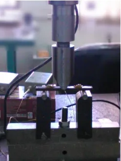
Bending tests were conducted in a properly calibrated three-point bending apparatus, with a span length of 70 mm, equipped with a deflection measuring device shown in Figure 1. A bar of rectangular cross section with dimensions according to Table 1, rests on two supports and is loaded by means of a loading nose midway between the supports. Modulus of elasticity of test samples was measured in accordance with ASTM D790-10 by Equation (1) [13].

3

B ₃

L m E =

4bd (1)

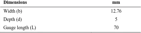
TABLE 1.Bending test sample dimensions

Dimensions mm

Width (b) 12.76

Depth (d) 5

(3)

where EB, L, b, d, and m are modulus of elasticity in bending, support span or gauge length, width and depth of beam tested, and slope of the tangent to the initial straight-line portion of the load-deflection curve of deflection, respectively. The experimental modulus of elasticity for different volume fraction of wood flour is tabulated in Table 2 as follows:

4. MODELING PROCEDURE

The modeling procedure of an RVE of wood flour composite is presented in this section. In this procedure, RVEs for volume fractions of 40%, 50%, and 60% have been made. Once designing of the RVEs for different volume fractions of interest are completed, they will go through some particular loading scenarios to determine their technical constants of elasticity via strain energy stored in the whole RVE [14] (Figure 2).

where in Figures 2a, b, c, d, and e are corresponding loading modes for evaluating longitudinal modulus E1, transverse modulus E2=E3, shear modulus in the plane of isotropy G23, shear modulus G12, and Poisson’s ratio

12

 , respectively. These constants will be subsequently used to calculate the material stiffness tensor for uni-directionally aligned short-fiber composites in accordance with Equation (5) which is the basis of future orientation averaging calculations.

Figure 1. Three-point bending apparatus used in this study for calculating modulus of elasticity of test samples

TABLE 2. Experimental values of modulus of elasticity for beech wood flour composites with different volume fractions of wood flour

Wood flour volume fraction (%) EB (GPa)

40 1.81

50 2.57

60 3.43

Figure 2. Schematic of five different loading scenarios in order to make an assessment of elasticity parameters of an RVE: E1 (a). E2=E3(b). G23 (c). G12 (d). 12 (e). [14]

The RVE consists of wood flour which completely embedded in a block of matrix. The flour considered as a cylinder with height of 30 micron and aspect ratio 1.5. Dimensions of matrix block is determined in a way that volume fraction of wood flour is satisfied [14]. The geometry characteristics of designed RVE are shown in Figure 3.

Therefore the volume fraction of the RVE will be calculated by Equation (2) as follows:

2

πr h

VF= ×100

a l

(2)

where in Equation (2), VF, r, h, a, and l are volume fraction of wood flour in percent, radius and length of wood flour in micron, width and length of block of matrix in micron as shown in Figure 3, respectively.

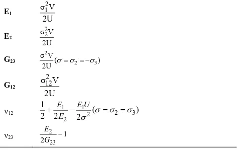
In Table 3, all of the equations which are necessary to assess elasticity constants are given. In Table 3, V is the total volume of the RVE and U is the strain energy acquired from FE analysis.

4. 1. Orientation Averaging Existing methods for predicting elastic properties of short-fiber polymer composites from fiber orientation tensors are based on the orientation function which is the average of a transversely isotropic stiffness tensor.

(4)

TABLE 3. Equations for assessing elasticity constants via strain energy procured from FEA

E1

2 1 σ V

2U

E2

2 2

σ V 2U

G23

2

2 3

σ V

( )

2U     G12

2 12

σ V 2U

12 1 1₂ 2 3

2 1

( )

2 2 2

E E U

E    

   

23

2 23

1 2

E

G 

These evaluations focus solely on average properties and have yet to include a quantitative measure of property variation. Recognizing the statistical nature of fiber orientations within the composite commonly defined through the fiber orientation distribution function [15]. In this investigation, finding an appropriate fiber orientation distribution function in order to assess a good estimation of wood flour reinforced composites is considered as a main scope. Hence, the orientation averaging approach will be presented in subsection 4.1.1. In subsection 4.1.2, the preferred orientation distribution function which results the best answers compared with experimental results is introduced.

4. 1. 1. Orientation Averaging Procedure This method was first time validated by Gusev et al. [16] through analyzing of composites with relatively low volume fraction of fiber about 15%, for some variant orientation states, the result of the mentioned study was that orientation averaging suggests precise prediction in engineering scales. The fundamental idea of the approach is presented: the fiber orientation is fully outlined by the direction unit vector p, shown in Figure 4 [17].

1

p =sin(θ) cos(φ)

(3)

2

p =sin(θ) sin(φ)

3 p =cos(θ)

An infinite series of orientation tensors delineates the orientation of a whole set of fibers. Because the fiber positioning is repeated, meaning a fiber oriented at angles (φ,θ) is identical from another one with angles (φ+π,θ+π), due to symmetry considerations, only the even second and fourth order tensors a2, a4 are pertinent. These are interpreted as:

Figure 4. A fiber along a unit directional vector p [15]

2π π

ij i j i j

0 0

a =<p p >=

 

p p Ψ(φ,θ) sin(θ)dθdφ

(4)

2π π ijkl i j k l i j k l

0 0

a =<p p p p >=

 

p p p p Ψ(φ,θ) sin(θ)dθdφ

where, ( , )  is the probability distribution function or in the other sense of the word, fiber orientation distribution function, identifying the fiber orientations in the composite [17]. This function should fulfil orthogonality condition as mentioned in Equation (4) [17]:

2π π l 0 0

Ψ(φ,θ) sin(θ)dθdφ=1

 

(5)

The elastic tensor property, <C>, of a random fiber composite can be obtained by averaging a transversely isotropic tensor property of an aligned fiber composite,

C (Equation (5)), over all directions, weighted by

orientation distribution function as Equation (6) [15]:

12 12

1 1 1

23 12

1 2 2

23 12

1 2 2

23

12

1

0 0 0

1

0 0 0

1

0 0 0

1

0 0 0 0 0

1

0 0 0 0 0

1

0 0 0 0 0

E E E

C

G

 

 

 

 

  

 

  

 

    

 

 

 

(6)

<C> =



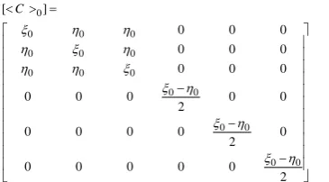
Ψ(p)dp (7)

According to [15], Equation (6) could be disintegrated in three distinguishable terms as Equation (7):

0 2 4

[          C ] [ C ] [ C ] [ C ] (8)

(5)

0

0 0 0

0 0

[ ]

0 0 0

0 0 0 0 0

2

0 0 0 0 0

2

0 0 0 0 0

2 C                            _       _       _      (9)

where, coefficients ξ₀ and η₀ are defined as [15]:

11 12 22 55

0 1

(3 4 8 8 )

15 C C C C

    

(10)

11 12 22 55

0 1

( 8 4 )

15 C C C C

    

where, [Cmn], m, n ∈ {1,2, … ,6}, is the (m,n) component of the uni-directional stiffness matrix [C₂] from Equation (7). [ C ₂]in Equation (11) is:

2 2 2 23 2 13 2 12 2

2

23 2 23 2 23 2 2 12 2 13 2

13 2 13 2 13 2 12 2 2 23 2

12 2 12 2 12 2 13 2 23 2 2

Aτ Bε -Cε 3a ε a ε a ε Bε Cτ -Aε a ε 3a ε a ε

-Cε -Aε -Bτ a ε a ε 3a ε C =

3a ε a ε a ε -Aη 3a η 3a η a ε 3a ε a ε 3a η -Cη 3a η

a ε a ε 3a ε 3a η 3a η Bη

             _{ } _      (11) 11 11 22 22 A=3a -1 B=3a +3a -2 C=3a -1

(12)

where, the coefficients ₂, ₂, and ₂ are given as:

11 12 22 55

2 6

ξ = (3C +C -4C +2C ) 42

(13)

11 12 22 23 55

2 1

η = (2C -4C -5C +7C +6C ) 42 2 2 2ξ τ = 3

2 2 2

1 ε = (ξ -6η )

3

And finally [ C ₄] will be given as Equation (14) in tensor form for the sake of conciseness as follows:









4 4 1 7 1 3 ijkl

ij kl ij kl kl ij ik jl il jk jk il jl ik

ij kl ik jl il jk

C

a a  a  a  a  a  a 

         _ _ _ _ _ _      _ _ _      (14)

where, _mn, m, n{1,2, … ,6}, is kronecker delta and

4

 is defined as Equation (15).

11 12 22 55

4 C 2C C 4C

     (15)

4. 1. 2. Fiber Orientation Distribution Function

The function of the form Ψ(θ, )=csin θ.cos_ 2n 2n__from [18] is chosen as fiber orientation distribution function, where n ∈N. Notice that n=0 yields the isotropic case, which fibers are randomly oriented all over the RVE. As the n increases the fiber orientation tends to orient along the x axis which results higher stiffness. This direction (x) agrees with the direction which melted WPC flows during the injection molding process. The constant c is chosen to satisfy the normalization condition [18].

4. 2. Boundary Conditions For the purpose of obtaining elastic constants of the RVE, it should go under some loading scenarios which have been described in detail in [14]. This loading modes can categorized in two basic groups which are loading under normal stresses e.g.

1 0 x

σ and loading under shear

stresses e.g.

1 2 0 x x



. The boundary conditions according to these basic types of loading are presented in subsequent subsections.

4. 2. 1. Subjected to 0₁ x

σ Consider the RVE shown in Figure 5. The boundary conditions must be set in such a way that the compatibility of the unit cell with neighboring cells in the infinite composite could be satisfied. For the loading case under normal stresses, in the absence of shear loading, the bottom edge of the RVE (x1-axis) was not allowed to move in the x2 -direction and the left edge (x2-axis) was not allowed to move in the x1-direction (Figure 5) [19, 20].

The right edge can have an equal amount of the displacement in x1-direction and the top edge can have an equal displacement in x2-direction, so the nodes on right edge must be coupled in the x3-direction. Similarly, the nodes Therefore, appropriate boundary conditions on the various edges of the RVE can be considered as [21]:

on the top edge must be coupled in the x1-direction [19].

(6)

1

1 1

0 x

x =0 x =a

u =0 and u = aε

(16)

2 2

2

0 x =b x x =0

v =0 and v = bε

3 3

3

0 x =c x x =0

w =0 and w = cε

where a, b, and c (which is not shown in Figure 5) are the three dimensions of the RVE shown in Figure 5 and u, , w,

1 0 x

ε ,

2 0 x

ε , and

3 0 x

ε are corresponding

displacements and strains along x1, x2 and x3 directions respectively [21].

4. 2. 2. Subjected to

2 3 0 x x



The nature of shear stresses is slightly more complicated than their direct counterparts. As summary, all boundary conditions for the unit cell under macroscopic stress

2 3 0 x x



are as follows [21]:

1 1

x =0 x =a

u = u = 0

(17)

2 2 2 2

x =0 x =0 x =b x =b

u = w = u = w = 0

2 3

3 3 3 3

0 x x

x =0 x =0 x =c x =c

u = v = u =0 and v =cγ

The matrix is assumed to be perfectly bonded to the fibers throughout the analysis. This requires satisfaction of the continuity of displacements and reciprocity of traction at the fiber-matrix interface:

f m

u =u , t +tf m0 (18)

where, superscript f and m denote fiber and matrix, respectively, and u and t are the displacement and traction vectors on the interface [19, 20].

5. RESULTS AND DISCUSSIONS

RVEs of interested volume fractions have been generated. A FEA (finite element analysis) was carried out using the FEA code and Proper boundary conditions have been imposed on RVEs in accordance with section 4. Consequently, stiffness tensors of beech wood flour composite specimens have been estimated using orientation averaging scheme by appropriate orientation distribution functions. In order to acquire these stiffness tensors, primarily, as mentioned before, an RVE of interested volume fraction of fiber goes through a loading scenario, demonstrated by Figure 2. Once this stage is done, all of Ccomponents will be computed by FEA code. By using orientation averaging scheme and evaluating [ C ₀],[ C ₂], and[ C ₄]according to

Equations 8, 10 and 12, and adding up these procured results commensurate with Equation (7), the final stiffness tensors which are exploited for prognosticating mechanical properties of WPC are acquired.

Three different orientation distribution functions which are discriminated with each other by their n values (Table 4), have been evaluated in this study and corresponding stiffness tensors were calculated and the orientation distribution function with best answer fitting to the experimental results is selected as a best function to predict stiffness properties of wood flour composites. C3D8R, C3D6, and C3D4 elements have been employed for FE analysis and finer meshing strategy is used at the places which loads are exerted.

One of the best features of this method is benefiting from orthodox orientation distribution functions to have a relatively impeccable anticipation of WPC mechanical property. There are so many functions which may fulfill conditions like orthogonality condition but few of them can result in an accurate answer as a corollary of a right decision of choosing appropriate functions. It is conceivable that finding suitable function in WPCs with low volume fraction of fiber, is not a major problem. In these amount of volume fractions of fiber, even selecting isotropic distribution of fibers in matrix, might result in good prediction, but in higher volume of fractions, like more than 40% of wood, the issue is completely different. As the volume fraction of fiber elevates, discrepancy between experimental and predictions answers ascends. Most of FEA methods like Random Sequential Adsorption and Monte Carlo codes fail to have an accurate prediction in such high volume fractions. Therefore, finding a method to compensate this lacuna is in a great interest.

The most important facet which is obvious in selecting n=0 (considered as isotropic distribution of wood particles in matrix) for orientation distribution function, is a considerable relative error which increases more and more as volume fraction of wood increases, compared to functions with higher n (n=1, n=2). By choosing with higher value of n, the accuracy of the answers gets better and the best predicted value is acquired at n=2, with lowest relative error in highest volume fraction of wood at 60%.

TABLE 4. Orientation distribution functions as a function of n

n Ψ(θ, )=Csin θ.cos 2n 2n

0 1

4

1 3sin θ.cos2 2

4π 

2 5sin θ.cos4 4

(7)

The strain energy density of different loading modes, according to [14] is obtained as mentioned before and the stiffness tensors components for different volume fractions and different fiber orientation distribution functions are presented in Tables 5, 6, and 7.

Predicted Young’s modulus were obtained by orientation averaging, employing three different orientation distribution functions presented in Table 3, are shown in Table 8 in comparison with experimental results. As it is obvious from Table 8. isotropic distribution of flour in matrix (n=0) yields farthest answers, compared to experimental results.

TABLE 5. Stiffness tensors components for the volume fractions of interest withΨ(θ, )=1

4π



VF (60%) VF (50%)

VF (40%) Cijkl (GPa)

3.91 3.27 2.75 1111 1.70 1.62 1.52 1122 1.70 1.62 1.52 1133 1.70 1.62 1.52 2211 3.91 3.27 2.75 2222 1.70 1.62 1.52 2233 1.70 1.62 1.52 3311 1.70 1.62 1.52 3322 3.91 3.27 2.75 3333 1.10 0.82 0.61 2323 1.10 0.82 0.61 3131 1.10 0.82 0.61 1212

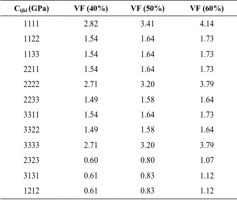
TABLE 6. Stiffness tensors components for the volume fractions of interest with_{Ψ(θ, )=} 3_{sin θ.cos}2 2

4π

 

VF (60%) VF (50%)

VF (40%) Cijkl (GPa)

4.14 3.41 2.82 1111 1.73 1.64 1.54 1122 1.73 1.64 1.54 1133 1.73 1.64 1.54 2211 3.79 3.20 2.71 2222 1.64 1.58 1.49 2233 1.73 1.64 1.54 3311 1.64 1.58 1.49 3322 3.79 3.20 2.71 3333 1.07 0.80 0.60 2323 1.12 0.83 0.61 3131 1.12 0.83 0.61 1212

TABLE 7. Stiffness tensors components for the volume fractions of interest with_{Ψ(θ, )=}5_{sin θ.cos}4 4

4π

 

VF (60%) VF (50%)

VF (40%) Cijkl (GPa)

4.40 3.54 2.91 1111 1.66 1.61 1.51 1122 1.66 1.61 1.51 1133 1.66 1.61 1.51 2211 3.80 3.20 2.72 2222 1.64 1.57 1.42 2233 1.66 1.61 1.51 3311 1.64 1.57 1.48 3322 3.80 3.20 2.72 3333 1.07 0.81 0.61 2323 1.04 0.79 0.58 3131 1.04 0.79 0.58 1212

TABLE 8. Predicted Young’s modulus of beech wood flour-PP composites, using different fiber orientation distribution functions as a function of volume fraction in comparison with experimental data

Beech wood flour volume fraction (%) n

Predicted E (GPa) Experimental E (GPa) Relative Error (%) 40

0 1.67 1.81 -7.73

1 1.71 1.81 -5.52

2 1.80 1.81 -0.55

50

0 2.20 2.57 -14.40

1 2.28 2.57 -11.30

2 2.46 2.57 -4.30

60

0 2.88 3.43 -16.03

1 3.02 3.43 -11.95

2 3.39 3.43 -1.17

With this distribution of flour in matrix, as volume fraction of flour increases, the less precision in predicting of Young’s modulus is obtained. This can be related to creating of voids within the matrix as flour volume fraction ascends. As the value of n increases to one, the predicted stiffness increases, as expected, because fibers tends to have orientation along melt flow in compression molding procedure, therefore better answers in comparison with the case n=0 are obtained. The best predicted Young’s modulus is acquired by choosing n=2 for fiber distribution orientation function. This means that fiber distribution function

4 4

5

Ψ(θ, )= sin θ.cos 4π

  is the best function in estimating

(8)

applications. Regarding all these facts, predicting stiffness property of short fiber composites with satisfactory precision in high volume fraction of fiber will be reachable but choosing a good fiber distribution function which results good prediction is going to be a major challenge. Hence, further study should be done on variant WPC samples in order to defining the best fiber distribution functions which result the best answers fitting experimental results with lowest discrepancies. Afterwards the best fiber distribution functions which yields best answers can be collected and clustered in a handbook

.

6. CONCLUSION

Orientation averaging approach has been employed in order to predict the stiffness properties of beech wood flour-PP composites. An RVE of interested volume fraction was generated and FE analysis was performed in order to evaluate stiffness tensors, according to the three different fiber distribution functions. By considering isotropic distribution of the wood flour in matrix, the predicted Young’s moduli do not have enough precision to estimate the stiffness of WPC specimens. Choosing n=0 for fiber distribution function has another consequence which compromises the precision of the answers compared to the experimental results in higher volume fractions of wood flour. Hence, as the volume fraction of wood flour increases, the distance between predicted and experimental results rises, resulting greater relative error. It has been shown

that the Ψ(θ, )= 5sin θ.cos4 4 4π

  results the best answers

in comparison with experimental data in predicting stiffness property of beech wood flour-PP composites. Another aspect of selecting this fiber distribution function is its precision in finding better answers as volume fraction of wood flour escalates in such a way that relative error can be neglected in comparison with isotropic distribution of the wood flour.

7. REFERENCES

1. Wolcott, M.P. and Englund, K., "A technology review of wood-plastic composites", in 33rd International particleboard/composite materials symposium. Vol., No. Issue, (1999), 103-111.

2. Segerholm, K., "Characteristics of wood plastic composites based on modified wood: Moisture properties, biological performance and micromorphology", KTH Royal Institute of Technology, (2012),

3. Gibson, R.F., "Principles of composite material mechanics, CRC press, (2016).

4. Kalaprasad, G., Joseph, K., Thomas, S. and Pavithran, C., "Theoretical modelling of tensile properties of short sisal fibre-reinforced low-density polyethylene composites", Journal of

Materials Science, Vol. 32, No. 16, (1997), 4261-4267.

5. Facca, A.G., Kortschot, M.T. and Yan, N., "Predicting the elastic modulus of natural fibre reinforced thermoplastics",

Composites Part A: Applied Science and Manufacturing, Vol.

37, No. 10, (2006), 1660-1671.

6. Migneault, S., Koubaa, A., Erchiqui, F., Chaala, A., Englund, K. and Wolcott, M.P., "Application of micromechanical models to tensile properties of wood–plastic composites", Wood Science

and Technology, Vol. 45, No. 3, (2011), 521-532.

7. Advani, S.G. and Tucker III, C.L., "The use of tensors to describe and predict fiber orientation in short fiber composites",

Journal of Rheology, Vol. 31, No. 8, (1987), 751-784.

8. Nassehi, V., Hashemi, S. and Beheshty, M., "A numerical method for the determination of an effective modulus for coated glass fibers used in phenolic composites", International Journal

of Engineering, Vol. 13, No. 3, (2000), 1-10.

9. Okafor, E.C., Ihueze, C.C. and Nwigbo, S., "Optimization of hardness strengths response of plantain fibres reinforced polyester matrix composites (pfrp) applying taguchi robust resign", International Journal of Science & Emerging

Technologies, Vol. 5, No. 1, (2013).

10. Heydari, M. and Choupani, N., "A new comparative method to evaluate the fracture properties of laminated composite",

International Journal of Engineering, Vol. 27, No. 6., (2014),

1025-2495.

11. Todorovic, N., Popadic, R., Popovic, Z. and Dukic, U., "Bending strength and modulus of elasticity of thermally modified beech wood".

12. Stark, N.M., "Wood fiber derived from scrap pallets used in polypropylene composites", Forest Products Journal, Vol. 49, No. 6, (1999), 39-45.

13. Properties, A.S.D.o.M., "Standard test methods for flexural properties of unreinforced and reinforced plastics and electrical insulating materials, American Society for Testing Materials., (1997).

14. Modniks, J. and Andersons, J., "Modeling elastic properties of short flax fiber-reinforced composites by orientation averaging",

Computational Materials Science, Vol. 50, No. 2, (2010),

595-599.

15. Pan, Y., "Stiffness and progressive damage analysis on random chopped fiber composite using fem, Rutgers The State University of New Jersey-New Brunswick, (2010).

16. Gusev, A., Heggli, M., Lusti, H.R. and Hine, P.J., "Orientation averaging for stiffness and thermal expansion of short fiber composites", Advanced Engineering Materials, Vol. 4, No. 12, (2002), 931-933.

17. Iorga, L., Pan, Y. and Pelegri, A., "Numerical characterization of material elastic properties for random fiber composites",

Journal of Mechanics of Materials and Structures, Vol. 3, No.

7, (2008), 1279-1298.

18. Jack, D.A. and Smith, D.E., "Elastic properties of short-fiber polymer composites, derivation and demonstration of analytical forms for expectation and variance from orientation tensors",

Journal of Composite Materials, Vol. 42, No. 3, (2008),

277-308.

19. Ahmadi, I. and Aghdam, M., "A generalized plane strain meshless local petrov–galerkin method for the micromechanics of thermomechanical loading of composites", Journal of

Mechanics of Materials and Structures, Vol. 5, No. 4, (2010),

549-566.

20. Ahmadi, I. and Aghdam, M., "Micromechanics of fibrous composites subjected to combined shear and thermal loading using a truly meshless method", Computational Mechanics, Vol. 46, No. 3, (2010), 387-398.

21. Li, S., "Boundary conditions for unit cells from periodic microstructures and their implications", Composites Science and

(9)